Tempo inference¶

There is a link between the occurence of musical events and the passing of relative time: the interpretation of a duration of 1 beat depends on the current tempo which is infered from the occurence of musical events.

The tempo inference is based on an approach proposed by Edward W. Large and Mari Riess Jones in the article The dynamics of attending: How people track time-varying events. The basic idea is to maintain an internal clock within Antescofo that represents the passage of time in the musician. This clock synchronizes with the musical events produced by the musician while taking into account the tempo indications from the score. The coupling of this internal clock with the musician is controlled by two parameters that allow for making tempo inference more responsive or, conversely, imposing more inertia in the face of tempo changes.

The details of tempo inference are described below. Most of the time, these details can be ignored, but it is sometimes necessary to adjust the inference parameters to improve synchronization between the musician and the electronic response.

It should be emphasized that the inferred tempo is used by the listening machine to improve detection of the occurrence of the next musical event. Modifying the inference parameters modifies the calculated tempo, and its value can degrade the recognition of musical events. The default parameters are intended to be relevant in a wide variety of musical contexts. If the inferred tempo is not suitable for driving certain electronic processes, a solution that is often more appropriate is to impose an ad-hoc computed tempo on these processes, rather than changing the inference parameters.

Defining the expected tempo¶

The BPM specification¶

The tempo inference is initialized by the BPM specification that appear in the score.

This statment BPM is a static specification similar to a tempo specification in a traditional score and gives the musician's expected tempo . Nota Bene that the BPM indication does not set the tempo: the musician's interpretation may deviate from the score's specification.

The BPM specifications are only used to initiate the inference of the actual tempo. The actual performer's tempo is infered from the BPM specifications and the timing of the musical events. Its current value is available as the value of the variable $RT_TEMPO while the value of the BPM specification can be accessed at any point through the variable $SCORE_TEMPO. The inference process is explained below and makes possible the dynamic adaptation of the electronic processes to the actual interpretation of the performer.

A BPM specification can be qualified by the attribute @modulate which makes possible to take into account the actual performer's tempo in the prescribed change. For example, if the performer adopts a tempo of $67$ in the section defined at BPM 60 in the following score

    BPM 60
        NOTE 70 1/8
        NOTE 72 1/8
        NOTE 70 1
        NOTE 70 1/8 
        NOTE 72 1/8 
        NOTE 70 13/8
    BPM 55 @modulate
        NOTE 69 1/8 
        NOTE 67 1/8 
        NOTE 65 1/8 
        NOTE 63 1/8 
        NOTE 65 1/8 
        NOTE 72 1/8
        NOTE 70 10/8

then for the next section at BPM 55 @modulate, the expected tempo is $61.47 = 67/60*55$. Modulation is therefore multiplicative with a factor computed as the ratio between the actual tempo divided by the score tempo.

Static specification of continuously varying tempo¶

Specifying an accelerando or a deccelerando is a tedious task with BPM statements that requires the definition of a different tempo for each musical event. In addition, with this approach, the tempo is supposed to remain fixed in-between events.

It is possible to overide the BPM specification by a tempo curve using the command antescofo::musician_tempo. The tempo curve is specified by an arbitrary nim (the nim value must be positive or null). The command is evaluated dynamically but its effect is similar to the BPM statment: it defines the expected tempo but does not set it.

There is an other possible use for antescofo::musician_tempo besides the specification of accelerando/deccelerando: the nim defining the tempo curve may be derived from a previous performance (for instance during a rehearsal). So the the predictions of the listening machine will be more accurate, as they benefit from more precise information on the tempo to be adopted by the musician.

When the expected tempo is continuously varying, the variable $RT_TEMPO varies continuously between events, in accordance with the variation of the specified tempo curve, and adjusted at musician events as it is the case for @modulate¹.

Disabling the tempo inference¶

The tempo inference is switched off if the listening machine is switched off (using suivi 0) or with the special command

     tempo off    ; or tempo 0

this command stops the inference and the tempo used to interpret relative musician time and by the listening machine is fixed to the current tempo value. The inference can be switched on with

     tempo on     ; or tempo 1

Implicit setting of the current tempo to zero¶

If musical events are expected but not reported, the current tempo is set to zero after the non-reception of the next 8 events. This behavior is handy in automatic accompaniment: when the musician stop to play, the accompaniment stops also a little bit later.

This behavior his only enabled if the follower is activated. In following mode, it can be silenced with the command

    Antescofo::bypass_temporeset 1

This is useful when Antescofo is used as a sequencer². The behavior can be switched on with

    Antescofo::bypass_temporeset 0

Dynamic setting of the current tempo with antescofo::tempo¶

At any moment, the current tempo can be set to a given value using the command antescofo::tempo. But once it is set, it is then updated by the tempo inference algorithm.

Tempo updates¶

When musical events are notified by the listening module or by nextevent or nextlabeltempo commands, the tempo is updated. However, the tempo is not updated:

• when tempo inference is disabled with tempo

• when other transport functions (like antescofo::nextlabel) are used to notify the musical event,

• when the event notified by the listening machine is not the event that immediately follows the current event (i.e., in case of missed events),

• on the first two events in the score (because duration are hardly respected at the very beginning of the performance).

• after a jump,

• after a grace note

• after a silence

• after a BPM specification (the tempo is set to the specified tempo)

• after the explicit seting of the tempo value with antescofo::tempo

• if the event is flagged as not to be used in tempo inference (with attribute @NoSync)

In the case of continuous tempo, the tempo is adjusted at each instant to follows the prescribed tempo curve modulated by the tempo achieved by the performer. Modulation is computed only when the tempo is updated as defined above¹.

Principle of the tempo inference¶

The current tempo is used to predict the arrival time of the next event. When this event actually occurs, the difference $\Delta$ between the predicted and the actual arrival time is regarded as a prediction error, which is used to correct the estimated tempo. This error has several origins:

1. the 'natural' fluctuation of the human performance;

2. a phase estimation error (i.e., the musician and antescofo have a discrepancy on the time origin)

3. and/or a tempo estimation error (the current infered tempo is not the actual tempo of the musician).

These two estimation problems can be illustrated by the antescofo program below, which bypasses the listening machine and itself explicitly calculates the score advancement. The variable $p in the program represents the duration of one beat as specified in the score; $mu_p represents the adjustments to add to $p to achieve the performer's actual tempo; and $mu_phi is used to represent the difference between the anetscofo time origin and the performer's time origin (a phase).

suivi 0
Group EmulateMusicianProgression 
{
   @local 
     $p := 1    // ideal (score) period 
     $mu_p := 0.1,    // period correction
     $mu_phi := 0.08  // phase correction

   loop ($p + $mu_p) s {
       $mu_phi s antescofo::nextevent
    } 
}

BPM 60

EVENT 1
EVENT 1
EVENT 1
...

There is no way to compensate the performer's natural fluctuations because we have no viable model of it. If we neglect this variation, the difference $\Delta$ can be used to compute two corrective terms, one used to adjust the Antescofo idea of the musician phase and one to adjust the inferred tempo — both are needed even if the musician phase is not used in the timing of the electronic actions.

The coupling factors¶

The amount of correction to apply to adjust the infered tempo is controled by two parameters: the coupling factors $\eta_{\,\phi}$ and $\eta_{\,p}$. The inference is convergent if the infered tempo converges to the tempo of a perfectly steady musician. The larger the coupling factors, the faster the convergence. Conversely a low coupling factors results in slower convergence of the estimated tempo to the actual tempo, which can be seen as a latency in the tempo prediction.

A coupling factor of $0$ means no correction at all (i.e., the infered tempo stays at its initial value) while $\eta_{\,\phi} = 2$ and $\eta_{\,p} = 1$ denotes the greatest possible correction compatible with a convergent inference.

For technical reasons, the antescofo tempo inference is convergent if $0 < \eta_{\,\phi} < 2$ and $0 < \eta_{\,p} < 1$ and if the initial infered tempo is in $]T/2, 2.T[$ where $T$ is the actual tempo of the musician.

The relative values of $\eta_{\,\phi}$ and $\eta_{\,p}$ implicitly define which part of $\Delta$ is allocated to the real phase approximation and which part is allocated to the tempo approximation.

Optimal coupling factors for steady performances¶

The antescofo program below is used to emulate the musician's performance in a strictly controlled way, bypassing the listening maching and explicitly programming the advancement in the score. The tab $noise is used to 〝blur〞 the performance which ideally goes at 60 BPM. By adjusting this tab, we can control the amount of random fluctuations of the performance.

Group Progression 
{
   @local $noise := [ -0.00411715, -0.0311941, 0.0266952, -0.0244803, ...]
   @local $p := 1 ; ideal period 

   loop ($p + $noise) s {
       antescofo::nextevent
    } 
}

BPM 60

EVENT 1
EVENT 1
EVENT 1
...

The following figures show the infered tempo (in blue) and the instantaneous tempo (in green) for the same noisy performance with various coupling factors. Instantenous tempo is computed for each event simply by dividing the duration of that event (in beats) with the duration of that event (in minutes). Because of the noise, the instantaneous tempo fluctuates around 60 BPM: here the fluctuations are between 57.5 and 62.5, that is a variation of of $5$ BPM or $8.3\%$.

The coupling factor are imposed using specific antescofo commands described below. We will explain at the end of this section how to plot these figures automatically. Open these figures in another tab for a magnified view.

Clearly, a high coupling factor for the period correction follows too closely the random fluctuation. This is visible because for the high period coupling of the two lower figures, the deduced tempo (in blue) shows a greater fluctuation than the instantaneous tempo. This is explained by the fact that a lower instantaneous tempo is a sign of a possible decrease in the tempo of the musician, a trend that is followed by the inferred tempo, whereas it is simply a random fluctuation that will be contradicted at the next event (and vice-versa for an increase in instantaneous tempo).

So, in this situation it is better to chose a small period coupling factor. If we don't specify the coupling factor, the default coupling strategy infers the following tempo:

Optimal coupling factors for varying tempo¶

Now we change a little bit the setting by imposing an accelerando from $55$ to $70$ in 90 beats. Note that this tempo is not specified in the score. We modulate dynamically the progression using a tempo curve to emulate a performer who accelerates on a score that indicates a fixed tempo.

$tempo_curve := NIM {0 55, 90 70 "quad_in" }
Group Progression @tempo := $tempo_curve
{
   @local $noise := [ -0.00411715, -0.0311941, 0.0266952, -0.0244803, ...]
   @local $p := 1 ; ideal period 

   loop ($p + $noise) {
       antescofo::nextevent
    } 
}

BPM 60

EVENT 1
EVENT 1
EVENT 1
...

Using the same coupling factor as in the previous example, we obtain:

This time, a low period coupling factor is hard to keep up with variations in the musician's tempo. This is clearly visible for $\eta_{\,p} = 0.1$, $\eta_{\,\phi} = 1.7$. This is also visible with $\eta_{\,p} = 0.1, \eta_{\,\phi} = 0.2$: the initial estimation of 60 takes time (more than 10 beats) to converge from 60 to 55.

With a hight period coupling factor, Antescofo follow more closely the tempo's variations. But a low or a high phase coupling factor makes the infered tempo a little bumpy³.

The default coupling strategy gives the following result, which is a good compromise between the reactiveness and the smoothness of the infered tempo.

From coupling factor to coupling strategies¶

The two examples have been choosen to show that a given pair of coupling factor cannot give the best results in all musical situation. The good default behavior of Antescofo despite the different musical context, is possible because Antescofo automatically adapts the coupling factor as a function of $\kappa$, a measure of the randomness of the performance⁴.

This dynamic adaptation is called a coupling strategy and Antescofo proposes four predefined adaptation strategies that can be selected with the command

    antescofo::large_tempo_parameters  int

• 0 is the default one. It has been tuned to cover a majority of musical context and to be relevant in a large range of performance variations.

• 1 results in a more reactive inference: the infered tempo more closely follows the musician's variations;

• 2 produces a less reactive inference: the infered tempo follows with more inertia the musician's variations;

• 3 leads to an inference that is better to more random performances.

The results of the four predefined strategies on the last example are illustrated by the following figures:

Defining your own coupling strategy¶

If one of the prdefined coupling strategy does not fit your needs, you can define your own specific coupling strategy. However, consider that:

• As mentionned in the preamble of this chapter, tempo inference is used by the listening machine. Changing this inference may adversely affect the performance of the listening machine. An alternative is to compute dynamically a specific tempo for your electronic voice, which suits your need and takes into account the inferred tempo in your own way.

• Avoid over-optimizing tempo inference. There is a natural fluctuation in the performer's playing that cannot be taken into account by inference and will vary from one performance to another.

• You shouldn't look for ‟beautiful” (e.g., smooth) tempo curves for the same reason.

For instance, to compute a tempo that does not completely follow the performer's variation but stick also to the tempo specified in the score, you can weight the two with a linear combinaison:

Group Electronic1 @tempo := (2*$SCORE_TEMPO + $RT_TEMPO)/3
{
   ; ...
}

If you still want to develop your own coupling strategy, the rest of this section is for you, but you have been warned.

Characterizing the musical context¶

The coupling strategy gives the $\eta_{\,p}$ and $\eta_{\,\phi}$ to use in the Large & Jones algorithm, as a function of $\kappa$.

However, for a low-duration event, the performer is expected to be less accurate, so that for a given $\kappa$ the coupling factor $\eta_{\,p}(\kappa)$ and $\eta_{\,\phi}(\kappa)$ must be smaller than for an event of non-low duration. Low duration are less than $0.3$ seconds.

This means that we must in fact define four functions (the two coupling functions for low-duration event and the two coupling function for the other events). We simplify the problem by assuming functions with a specific shape: for low-duration event, they are piecewise constant with two pieces (as in the following figure, left) and for the other events, the are piece-wise linear with 4 pieces (as in the following figure, right):

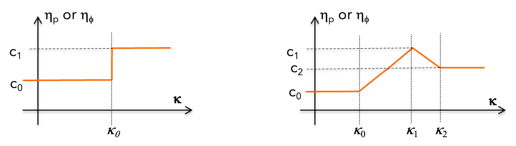
For low-duration event, a coupling function requires 3 parameters, and for non-low-duration event, we need 6 parameters. In addition, the duration (in seconds) of the time window used for the computation of the $\kappa$ parameter must also be specified.

This approach leads to $2* (3+6) + 1 = 19$ floating points parameters to define a specific coupling strategy. The commands listed in the rest of this paragraph can be used to specify all or only partially these parameters.

antescofo::large_tempo_parameters¶

The comamnd antescofo::large_tempo_parameters can be used to specify these 19 parameters as follow:

    antescofo::large_tempo_parameters p_s p_k p_l phi_s phi_k phi_l m k_1 p_1 k_2 p_2 k_3 p_3 phi_k1 phi_1 phi_k2 phi_2 phi_k3 phi3

where

• p_s defines $c_0$ the coefficient of $\eta_{\,p}()$ for low-duration event (see previous figure).

• p_k defines the $\kappa_0$ coefficient of $\eta_{\,p}()$ for low-duration event.

• p_l defines the $c_1$ coefficient of $\eta_{\,p}()$ for low-duration event.

• phi_s defines the $c_0$ coefficient of $\eta_{\,\phi}()$ for low-duration event.

• phi_k defines the $\kappa_0$ coefficient of $\eta_{\,\phi}()$ for low-duration event.

• phi_l defines the $c_1$ coefficient of $\eta_{\,\phi}()$ for low-duration event.

• mem defines the lenght of the time window used to compute $\kappa$. This duration is expressed in seconds. The window is a sliding window that ends with the current event.

• k_1 defines the $\kappa_1$ coefficient of $\eta_{\,p}()$ for large (non-low) duration event.

• p_1 defines the $c_1$ coefficient of $\eta_{\,p}()$ for large (non-low) duration event.

• k_2 defines the $\kappa_2$ coefficient of $\eta_{\,p}()$ for large (non-low) duration event.

• p_2 defines the $c_2$ coefficient of $\eta_{\,p}()$ for large (non-low) duration event.

• k_3 defines the $\kappa_3$ coefficient of $\eta_{\,p}()$ for large (non-low) duration event.

• p_3 defines the $c_3$ coefficient of $\eta_{\,p}()$ for large (non-low) duration event.

• phi_k1 defines the $\kappa_1$ coefficient of $\eta_{\,\phi}()$ for large (non-low) duration event.

• phi_1 defines the $c_1$ coefficient of $\eta_{\,\phi}()$ for large (non-low) duration event. Its value for the default coupling strategy is $1.77$.

• phi_k2 defines the $\kappa_2$ coefficient of $\eta_{\,\phi}()$ for large (non-low) duration event.

• phi_2 defines the $c_2$ coefficient of $\eta_{\,\phi}()$ for large (non-low) duration event.

• phi_k3 defines the $\kappa_3$ coefficient of $\eta_{\,\phi}()$ for large (non-low) duration event.

• phi_3 defines the $c_3$ coefficient of $\eta_{\,\phi}()$ for large (non-low) duration event.

The parameters have not been guessed but computed using an optimization procedure⁵. For information, the coefficients for the default coupling strategies are:

    /* p_s    */  0.16
    /* p_k    */  0.35
    /* p_l    */  0.25
    /* phi_s  */  0.85
    /* phi_k  */  1.2 
    /* phi_l  */  0.67
    /* mem    */  3.0
    /* k_1    */  1.0 
    /* p_1    */  0.5 
    /* k_2    */  2.60
    /* p_2    */  0.7
    /* k_3    */  6.0
    /* p_3    */  0.3 
    /* phi_k1 */  0.3 
    /* phi_1  */  1.87
    /* phi_k2 */  4.0
    /* phi_2  */  0.9 
    /* phi_k3 */  8.4
    /* phi_3  */  0.5    

Note that the same command antescofo::large_tempo_parameters is used to switch to one of the predefined coupling strategy (with one integer argument) or to specify the full 19 parameters of a specific coupling strategy.

The full specification of $\eta_{\,\phi}$ and $\eta_{\,p}$ is complex and additional commands can be used to ease the parameters specification when we want to redefine only some of the four coupling functions.

Command antescofo::tempo_sliding_mem¶

This command is used to change only the duration of the sliding window used to commpute $\kappa$ during the performance.

Command antescofo::small_tempo_phase_coupling_strenght¶

This command takes 0, 1 or 3 arguments to specify only the coupling function $\eta_{\,\phi}()$ for low-duration event:

• with no arguments, the coupling function is reset to its default value;

• with one argument, the coupling function is set to a constant function (that is, $c_0 = c_1$);

• with three arguments, the coupling function is defined by $c_0, \kappa_0, c_1$.

Command antescofo::small_tempo_period_adaptation_rate¶

This commands redefines the coupling function $\eta_{\,p}()$ for small duration event. The arguments are the same as those described for the previous command.

Command antescofo::large_tempo_phase_coupling_strenght¶

This commands redefines the coupling function $\eta_{\,\phi}()$ for large (non-small) duration event. The command takes:

• no argument: the function is reset to its default;

• one argument: the coupling function is set to a constant function (that is, $c_0 = c_1 = c_2$);

• six arguments: the coupling function is defined by the six $c_0, $kappa_0, c_1, $kappa_1, c_2, $kappa_2$.

Command antescofo::large_tempo_period_adaptation_rate¶

This commands redefines the coupling function $\eta_{\,\phi}()$ for large (non-small) duration event. The arguments are the same as those described for the previous command.

Monitoring and visualizing the tempo inference¶

Antescofo records various date used for the inference of the tempo during a performance. These data are available dynamically during the execuction via the function @performance_data(). See @performance_data for an example of how to use these data to plot the variation of the tempo.