Synchronization Strategies
The musician’s performance is subject to many variations from the score. There are several ways to adapt the timing of the electronic actions to this musical indeterminacy based on the specific musical context.
An electronic phrase is written that specifies delays between each action in a block (group, loop, whenever, curve, etc). Through specific attributes, a particular synchronization strategy defines the temporal evolution of this phrase depending on the musician's performance. More generally, a synchronization strategy specifies the temporal relationships between the actual timing of a sequence of actions and the actual timing of a sequence of events, see the previous section articulating time. The relevant synchronization strategy is determined by the musical context and is at the composer or arranger’s discretion1.
From a synchronization perspective, the musical performance can be summarized by two parameters: the musician's position (in the score) and the musician's tempo. These two parameters are computed by the listening machine from the detection in the audio stream of the events specified in the score. Synchronization takes them into account. The observed position in the score, for example, can be used to fix the position in the sequence; the tempo estimation can be used to compute the evolution of an action's position between two events and also to anticipate the arrival of future events.
An error handling strategy defines what to do with the action associated to an event that is never recognized (the origin of this “non-recognition” does not matter).
Temporal Scope
The system maintains a temporal scope for each running sequence of actions (groups, loops, curve, etc). A temporal scope defines
-
a local position (in beats): which represents the state of the progression when performing the sequence of actions;
-
and a local tempo (in beat per second): which represents the pace of the progression in the sequence of actions.
The synchronization attributes associated with a compound action define the temporal scope of the action relative to another temporal scope. By default, the referenced temporal scope comes from the actual musician's performance. But it is possible to specify another using the @tempo attribute or using the @sync attribute referring to a variable introduced by a @tempovar declaration.
In absence of specifications, a temporal scope is inherited from the enclosing compound action. The sequence of actions at top-level, are implicitly synchronized with a @loose synchronization strategy with the musician (cf. below).
Getting the tempo and the position of an arbitrary temporal scope
Two functions can be used to query the current tempo and the current position of an arbitrary temporal scope: @local_beat_position and @local_tempo. Without argument, these function returns the lcoal position and the local tempo of the temporal scope under which the function is called.
A temporal scope is linked to each exe. So the two previous functions may take an exe as an optionnal argument. When present, the local tempo or the local position refers to the current tempo and position of the temporal scope linked to this exe.
Two additionnal function can be used to convert a duration from local beat into seconds, or from seconds into local beats, assuming that the duration starts immediately. Note that because the tempo is dynamic, the conversion may return a different amount of beats or seconds following the date of the conversion. See @seconds_in_beats_from_now and @beats_in_seconds_from_now.
The following snippet shows how to plot (with @gnuplot the variation of a tempo and the progression of a local position computed from the assignment of a tempovar
Synchronization Attributes
The synchronization attributes are described below. They define how the position and tempo in the sequence of actions depends of the musician’s position and tempo:
-
@loose uses only the musician's estimated tempo to synchronize the actions;
-
@tight primarily uses the position information to synchronize the actions;
-
@target is an intermediary between tight and loose strategies, aimed to dynamically and locally adjust the tempo of a sequence for a smooth synchronization with anticipated events.
When both information of tempo and information of position are used, they can be contradictory (e.g., an event occurs earlier or later than anticipated from the tempo information). Two approaches are possible following the priority given to one parameter or the other. They are specified using the @conservative and @progressive attributes.
Finally, the synchronization mechanisms can be generalized to refer to the updates of an arbitrary variable instead to the musical events. The attribute @sync and the declaration @tempovar are used in this case.
Only one synchronization can be specified:
-
the synchronization attributes @sync, @tempo, @loose, @tight and @target are mutually exclusive;
-
@progressive is exclusive from @conservative but they can be combined with @target and @tight synchronization strategies;
-
@latency can be used to correct some latency problems, independently of the chosen synchronization strategy;
-
@ante and @post are experimental features not described here.
If no synchronization attribute are specified, then the corresponding group is @loose.
Loose Synchronization
Once a ‟loose” group is launched, the scheduling of its sequence of relatively-timed actions follows the real-time changes of the tempo from the musician. This synchronization strategy is the default one but an explicit @loose attribute can be used. The implicit top-level group that encompasses the sequence of actions linked to a musical event is loose by default (this can be changed using the top_level_groups_are_tight command.
The @loose attribute can be followed by a list of events: in this case, the change in the musician's tempo is considered only at these events (else they are considered on each musical event).
The figure below attempts to illustrate this within a simple example: the diagram shows the ideal performance or how actions and instrumental score is given to the system. In this example, an accompaniment phrase is launched at the beginning of the first event from the human performer. The accompaniment in this example is a simple group consisting of four actions that are written parallel (and thus synchronous) to subsequent events of the performer in the original score.
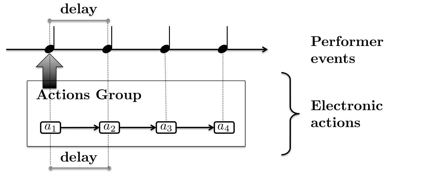
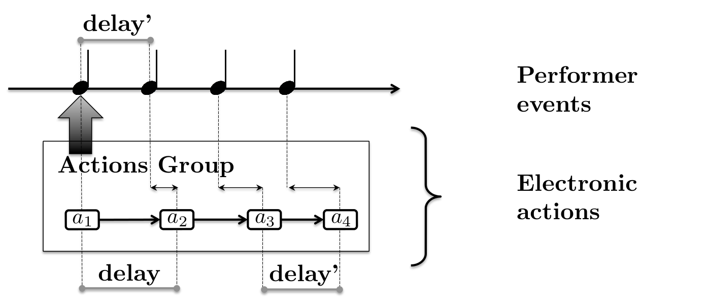
In a regular score following setting (i.e., correct listening module) the action group is launched in synchrony with the onset of the first event. For the rest of the actions, however, the synchronization strategy depends on the dynamics of the performance. This is demonstrated in the diagram below where the performer hypothetically accelerates the consequent events in the score.
In this diagram the performer hypothetically decelerates the consequent events in the score.
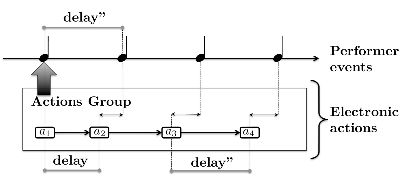
In these two cases, the delays between the actions will grow or decrease. The tempo inferred by the listening machine converges towards the actual tempo of the musician. Therefore, the delays, which are relative to the inferred tempo, will also converge towards the delay between the notes observed in the actual performance.
So, this synchronization strategy ensures a fluid evolution of the actions launching but it does not guarantee a precise synchronization with the events played by the musician. Although this fluid behavior is desired in certain musical configurations, there is an alternative synchronization strategy where the electronic actions will be launched as close as possible to the events' detection.
Tight Synchronization
If a group is @tight, its actions will be dynamically analyzed to be triggered not only using relative timing but also relative to the nearest event in the past. Here, the nearest event is computed in the ideal timing of the score.
The @tight attribute without parameters considers all musical events
to find the nearest event in the past. If parameters are provided, with
the syntax
@tight := { label₁, label₂, ... }
only the musical events refered by their labels are considered.
Tight groups allow the composer to avoid segmenting the actions of the group into smaller segments with regards to synchronization points and provide a high-level vision during the compositional phase. A dynamic scheduling approach is adopted to implement the behavior. During the execution the system synchronizes the next action to be launched with the corresponding event.
The implicit group that encompasses the sequence of actions linked to a musical event, uses the @loose synchronization strategy. This behavior can be changed to generate @tight groups by specifying the top_level_groups_are_tight keyword at the begining of the score (the change of behavior is global for the entire score).
Note that the arbitrary nesting of groups with arbitrary synchronization strategies do not always make sense: a @tight group nested in a @loose group has no well defined triggering event (because the starts of each action in the group are supposed to be synchronized dynamically with the tempo). All other combinations are meaningful. To acknowledge that, groups nested in a @loose group are @loose even if it is not enforced by the syntax.
Target Synchronization
In many interactive scenarios, the required synchronization strategy lies “in between” the @loose and @tight strategies. Through the @target attribute, Antescofo provides two mechanisms to dynamically and locally adjust the tempo of a sequence for a smooth synchronization.
-
static targets rely on the specification of a subset of events to take into account in the tempo adjustment, while
-
dynamic targets rely on a resynchronization window.
Static Targets
In some cases, a smooth time evolution is needed, but some specific events are temporally meaningful and must be taken into account. For example, this is the case when two musicians plays two phrases at the same time: they usually try to be perfectly synchronous (tight) on some specific events while other events are less relevant. These tight events can correspond to the beginning, or the end of a phrase or to other significant events commonly referred to as pivot events or attractors. Antescofo lets the composer list pivot events for a given block. During the performance, the local tempo of the block is dynamically adjusted with respect to the actual occurrence of these pivots, cf. figures below. In the following example:
          NOTE 60 2.0
              group @target := {e5, e10}
              {
                   actions ...
              }
              actions ...
          NOTE 45 1.2 e5
              actions ...
          NOTE 55 1.2 e10
the local tempo of the group will be computed depending on the
successive arrival estimations of events e5 and
e10. Notice that the pivots are referred to by their
label and listed between braces.
The second syntax a %% b is used to specify that the pivots are the
event located at \textrm{current position} + a * n + b beats (for n
\in \mathbb{N}).
The computed tempo aims to converge the position and tempo of the sequence of actions to the position and tempo of the musician at the anticipated date of the next pivot. The tempo adjustment is continuous: it follows a quadratic function of the position and the prediction is based on the last position and tempo values notified by the listening module, cf. figure below. This strategy is smooth and preserves the continuity of continuous curves.
Dynamic Target
Instead of declaring a priori pivots, synchronizing positions can be dynamically viewed as a temporal horizon: the idea is that the position and tempo of the block must coincide with the position and tempo of the musician at some date in the future. This date depends on a parameter of the dynamic target called the temporal horizon of the target. This horizon can be expressed in beats, seconds or number of events into the future. It corresponds to the necessary time to converge if the difference between the musician and electronic positions is equal to 1 beat.
In the following example:
          NOTE 60 2.0 e1
          group @target := [2s]
          {
                  actions ...
          }
the tempo and the position of the actions converge to the tempo and the
position of the musician. The convergence date is not an event (as in
static target) but is fixed by the following property: a difference of 1
between the position of the actions and the position of the musician is
corrected in 2 seconds. The syntax [2] is used to
specify a horizon in beats and [2#] to define a horizon
in number of events.
A small time horizon means that the difference between the position of action and the position of the musician must be reduced in a short time. A bigger time horizon allows for more time to lessen the difference. Notice that the relationship between the difference in position and the time needed to bring it to zero is not linear. As with static target synchronization, when a new event is detected, durations and delays are computed according to a quadratic function of the position. The date at which (position, tempo) converges only depends on the difference between the musician and electronic positions.
This strategy is smoother than static targets since the occurrence of events are used only to compute the anticipated synchronization in the future.
Comparison between @loose, @tight and dynamic @target
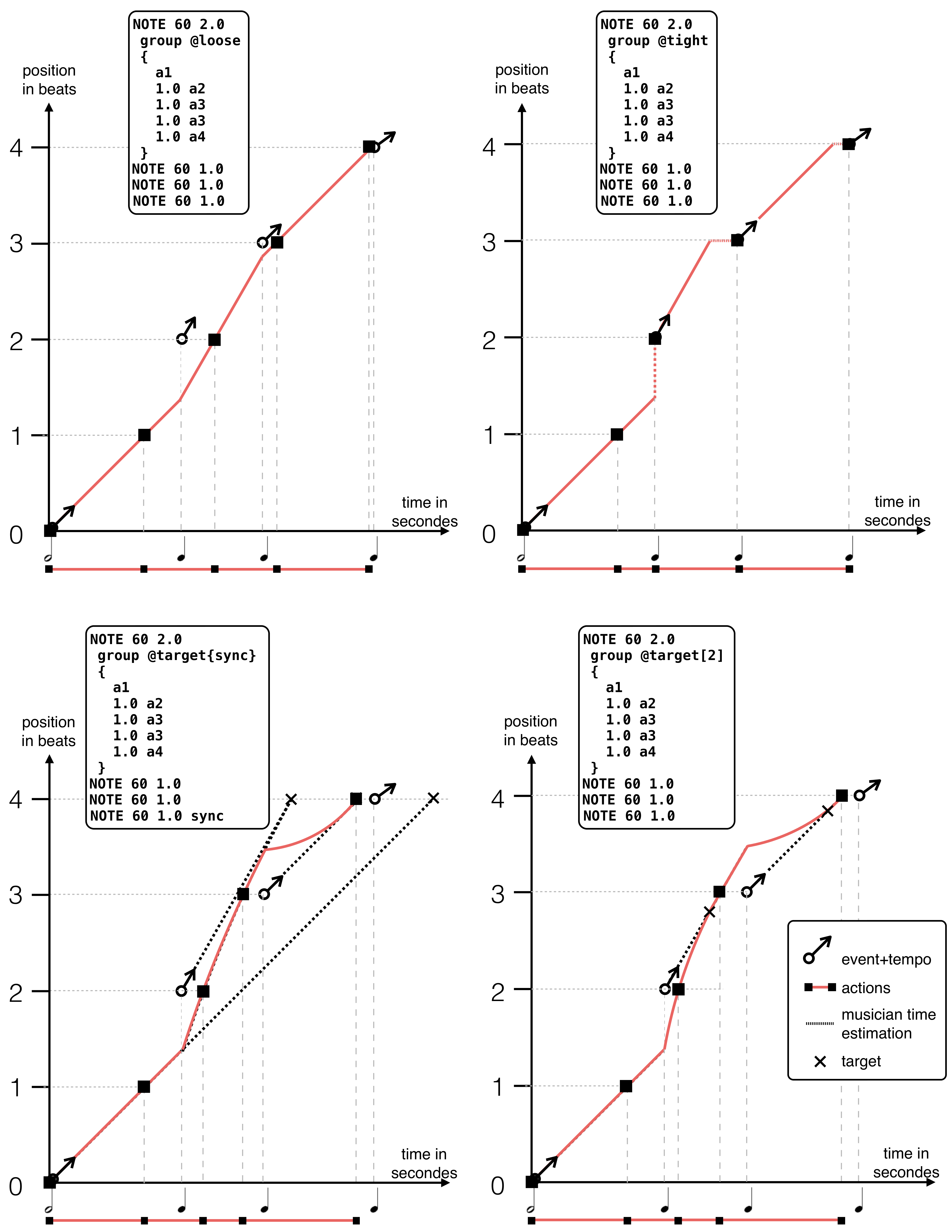
The figures below represent temporal evolution of an electronic phrase with several synchronization strategies. The time-time diagrams show the relationship between the relative time in beats andabsolute time in seconds2. The musical events are represented by vectors whose slopes correspond to the tempo estimation. The actions are represented by squares and the solid line represents the flow of time in the group enclosing these actions. From left to right and top to bottom, the strategies represented are : @loose, @tight, @target, @target [2]. There is an illustrative patch that compares the effects of synchronization attributes1.
How to Compute the Position in the Event of Conflicting Information
The @conservative and @progressive attributes parameterize the computation of the position of the musician in the synchronization strategy. They are relevant only for the @tight and @target strategies where both events and tempo are used to estimate the musician’s position.
-
With the @conservative attribute, the occurrence of events is trusted more than the tempo estimation to compute the musician’s position. So, when the anticipated date of an event is reached, the computed position is stuck until the occurrence of this event.
-
With @progressive attribute (the default), the estimation of the position will continue to advance even if the forecasted event is not detected.
Several system variables are updated by the system during real-time
performance to record these various points of view in the position
progression. They are used internally but the user can access their
values. Variable $NOW corresponds to the absolute date of the “current
instant” in seconds. The “current instant” is the instant at which the
value of $NOW is required.
The variables $RNOW and $RCNOW are estimations
of the current instant of the musician in the score expressed in
beats. At the beginning of a performance,
$NOW = $RNOW = $RCNOW
At other instants during the performance, let e_n be the last decoded event by the listening machine at time NOW_n, e_{n+1} the following event, p_n and p_{n+1} be their relative position in beats in the score, and del be the delay in beats since the detection of e_n. These variable are linked by the following equations:
where $RT_TEMPO is the last decoded tempo (in BPM) by the
listening machine. Then
`:::antescofo $RNOW` $\: = min($ `:::antescofo $RCNOW` $, \; p_{n+1})$
Notice that the $RNOW and $RCNOW values differ
when the estimated date of the next event is exceeded: $RNOW corresponds to the conservative notion of time progression and
remains at the same value until an event is detected, whereas the
variable $RCNOW corresponds to the progressive notion
of time progression and continues to grow following the tempo.
From a musical point of view, the position estimation with variables is more reliable when an event is missed (the musician does not play the note or the listening module does not detect it) but sometimes the value has to “go back” when the prediction is ahead.
Specifying Alternative Coordination Reference
Explicit tempo specification @tempo
The tempo local to a sequence of actions can be specified by an expression. This makes the local position and the tempo of the sequence completely independent to that of the musician. For example:
group @tempo := 70 { ... }
will execute the child actions with a tempo of 70. The tempo can be
defined by an expression. The variables of the expression are watched,
much like the variable in the expression of a whenever. When these variables are updated, the expression is
reevaluated, giving a new tempo value which is used to reevaluate
on-the-fly all the pending delays
Here is an example:
Curve C1 @grain 0.05s
{  $t1 { {60} 5 {180} 5 {60} } }

Group G1 @tempo := $t1
{
   @local $x
   $x := 0
   Loop L 0.1 {
        $x := $x + 0.1
    plot $NOW " " $x "\n"
   }
}
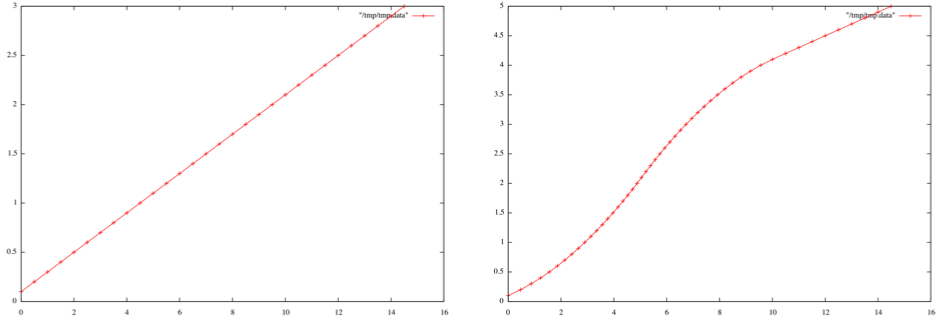
The values of the variable $x in the loop are plotted in
relative time at the left, and in physical time at the right. The linear
progression in relative time is transformed into a quadratic progression
made of two parabola, because the tempo variation is defined by a
piecewise linear function implemented by Curve C1 which
goes from 60 to 180 and back to 60.
Synchronization on a temporal variable with @sync
The synchronization mechanisms of a sequence of actions with the stream of musical events (specified in the score) has been generalized to make possible the synchronization of a sequence of actions with the updates of a variable. The variable can be updated internally in the computation specified by the score or from the external environment (for example with setvar or with OSC messages).
Such variables are global variables introduced using the
@tempovar declaration:
@tempovar $v(60, 2)
An update acts then as an event of duration 2 with a specified BPM of
60. The second argument of the declaration defines the increase in
the “position of $v” each time the variable is updated.
The first argument defines the initial “tempo” associated to this
variable. This tempo corresponds to the expected pace of the
updates. The position and tempo of a tempovar can be accessed using
the dot syntax, cf. temporal variable.
The attribute @sync is used to specify the synchronization of a sequence of action with the update of a variable. For instance:
          Curve C
          @sync := $v,
          @target := [10],
          @action := ...
          {
               $pos { {0} 5 {1} }
          }
specifies that the curve C must go from 0 to 1 in 5
beats, but these beats are measured in the time reference associated to
the temporal variable $v. In addition, the relation
between the current position in the curve and the position of the musician
is specified using a dynamic target strategy.
Latency Compensation
Latency compensation is an experimental feature. When attribute
@latency := 30ms is specified for a sequence of actions, the
runtime tries its best to anticipate the launch of each action by 30
milliseconds.
The anticipation is not guaranteed: it is taken on the delay preceding the actions in the sequence. So if the first action in the sequence is launched with no delay, the 30 ms cannot be compensated.
-
The interested reader will find on the forum at https://discussion.forum.ircam.fr/t/synchronization-strategies-examples/ a patch that can be used to compare the effect of the various synchronization strategies, including the synchronization on a variable. ↩↩
-
Read section the fabric of time for the notion of time-time diagrams. ↩