The Fabric of Time
Music as a Collective Performance
Antescofo tackles two fundamental problems of mixed music defined as the association in live performance (in the context of written music) of human musicians and computer mediums interacting in real-time:
-
music as a performance,
-
and performance as a collective process.
The first point refers to the divide between the score and its realization. Usually, notation does not specify all of the elements of music precisely, which leaves welcomed space for interpretation. The score can be thought of as a set of constraints that must be fulfilled by the interpretation but many score's incarnations may answer these constraints. The interpretation matters, conveying some meaning and assigning significance to the musical material. It is the performer's responsibility to choose/implement one of these possible incarnations. In doing so, the performer takes many decisions based on performance practice, musical background, individual choices and also because he is part of an ensemble: the music is played together with other musicians and the collective will dramatically affect the interpretation (our second point).
These two points challenge mixed music: how should various prescriptions of rhythm, tempo, dynamics and so on, be precisely realized within their permissible ranges by a computer? Computers cannot make these decisions out of the blue and, furthermore, have to take the other performers into account.
We restrict the rest of the discussion to the temporal relationships between various musical elements (to fix the idea, think about tempo). We qualify the temporal relationships specified in the score as potential and their realization in a performance as actual. A complete specification of the temporal relationships can be completely fixed by the composer, that is written in the score and definitive: the potential relationships are exactly the actual ones. For instance, it means that the tempo of the electronic action is explicitly specified in the score and implemented exactly during the performance. The interpretation problem is then avoided (there is no difference between potential and actual time), but then the human performer does not play with the machine: he or she has to follow the machine. This is no different from playing with a prerecorded tape, whereas the whole point of mixed music is to reintroduce the interpretation for the electronic part and to allow live interaction.
The obvious alternative is to let the composer to fix the interpretation but relatively to the interpretation of the performer. In this way, performers and computers play together, and there is still room for the human performer's interpretation. The situation is pictured below. For example, the electronic actions must follow the actual tempo of the performer, not the potential tempo possibly specified in the score.
This approach corresponds to a big shift of paradigm in mixed music and score following: electronic actions are not triggered on the occurrence of some musical events, but rather the timeline of the electronic is aligned (synchronized) with the timeline of the performer.
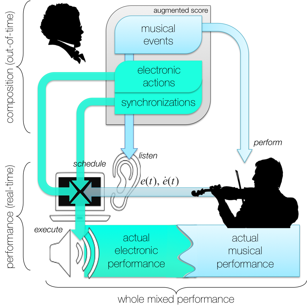
Antescofo follows this approach for temporal relationships. To implement it, Antescofo introduces several kinds of time:
-
the potential time expressed in the score
-
the actual time of the musical events performed on stage
-
the actual time of the electronic actions implemented in real time.
and requests the composer to specify their relationships. These relationships, expressed as synchronization strategies, are presented in the paragraph articulating time below and discussed at length in section Synchronization Strategies.
The Potential Score Time
The augmented score contains enough information to give a potential date to each event and action. These dates are specified through two pieces of information: the duration of each musical event and the tempo at each position in the score. The potential dating specified in the score can be represented as a curve picturing the advancement of the position in the score with respect to the passing of the physical time. See the plot below where the position in the score is measured in beats.
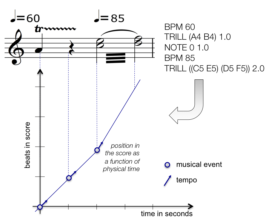
The occurrence of a musical event, represented by a circle and a vector, is used to give the tempo at this event. The vector represents a quantity measured in beats per second. The knowledge of the tempo can be used to compute the advancement in the score between two events, hence the potential date of each electronic action even if they are not synchronized with an event. For the sake of the simplicity, we suppose that the tempo is constant between two events1.
We call the previous map a time-time diagram because it relates the (potential) time in the score (in beats) with the physical time (in seconds). The previous map is completely defined by the set of pairs (position of event, tempo at event) $$ \bigl \{ \; (position_1, tempo_1), \; (position_2, tempo_2), \dots \; \bigr \} $$ which formalizes what we called ‟time” in the previous paragraphs. The potential time extracted from the score enjoys an important property:
A consequence is that the time-time diagram of potential time is a continuous curve.
The Actual Musician Time
During the performance, musicians interpret the score with precise and personal timing, while the potential score time (in beats) is evaluated into the physical time (measurable in seconds). For the same score, different interpretations lead to different temporal deviations, and musician's actual tempo can vary drastically from the nominal tempo marks. This phenomenon depends on the individual performers and the interpretative context.
The passing of time for the performer can be observed through the production of the musical events, so the information is restricted to the date of the occurrence these events. However, there are several methods to estimate the current tempo from the dating of the past events. The Antescofo approach is based on a study by Large and Jones2 but other approaches may still be relevant. In other words, the actual time of the musical events can be defined by a set of triples (date of event, position of event, tempo): $$ \bigl \{ \; (date_1, position_1, tempo_1), \; (date_2, position_2, tempo_2), \dots \; \bigr \} $$
From this information, a time-time diagram can be built to represent the passing of time for the performer (during the performance). But such diagrams will be merely formalities. There are indeed several ways to interpolate the positions between two events but no privileged way to choose one against the other, because there is no observation besides the musical events.
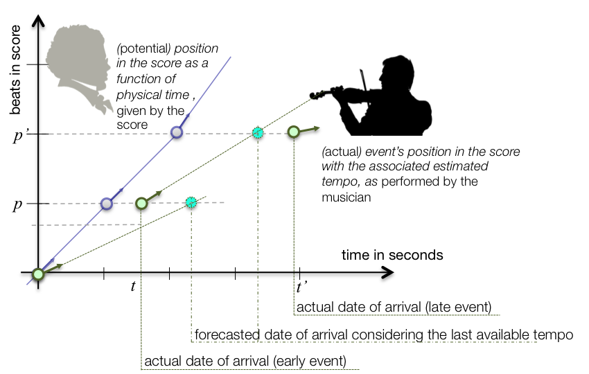
However, the tempo estimation at a particular event can be used to forecast the arrival of the next event3. The actual arrival may happen earlier or later than the predicted one: So, the relation between the actual position and the actual tempo is non-newtonian: the integration of the actual tempo gives only an approximation of the actual position.
This approximation can be seen as the result of the indetermination of the actual tempo at any instant. We advocate that this approximation is of a more fundamental nature: there is a divide between instantaneous discrete events (the onset of a note) and a general pace fixing the elapsing of a duration. The latter is a global and averaged quantity which does not prohibit the performer to advance or to postpone locally the occurrence of an event. Furthermore, the value of the tempo cannot be checked in between events.
Articulating Time
A unique feature of Antescofo is that it explicitly considers a time reference dedicated to the scheduling of the electronic actions. This time reference is specified by the composer and is dynamically computed during the performance, with respect to the potential time specified in the score and the actual time of the performer. This time-reference corresponds to a time-time map which is used to interpret beat positions, delays and durations involved in the actions.
This time reference is called a temporal scope. A temporal scope can be associated to each sequence of actions. By default, a sequence of actions inherits the temporal scope of its enclosing sequence of actions.
A temporal scope is defined by a synchronization strategy which defines how to ‟fill the gap” between the actual occurrence of events. There is a whole spectrum of synchronization strategies following the use of the information of position and the information of tempo. The interested reader will find a patch that can be used to compare the effect of the various synchronization strategies on a sequence of actions at this page.
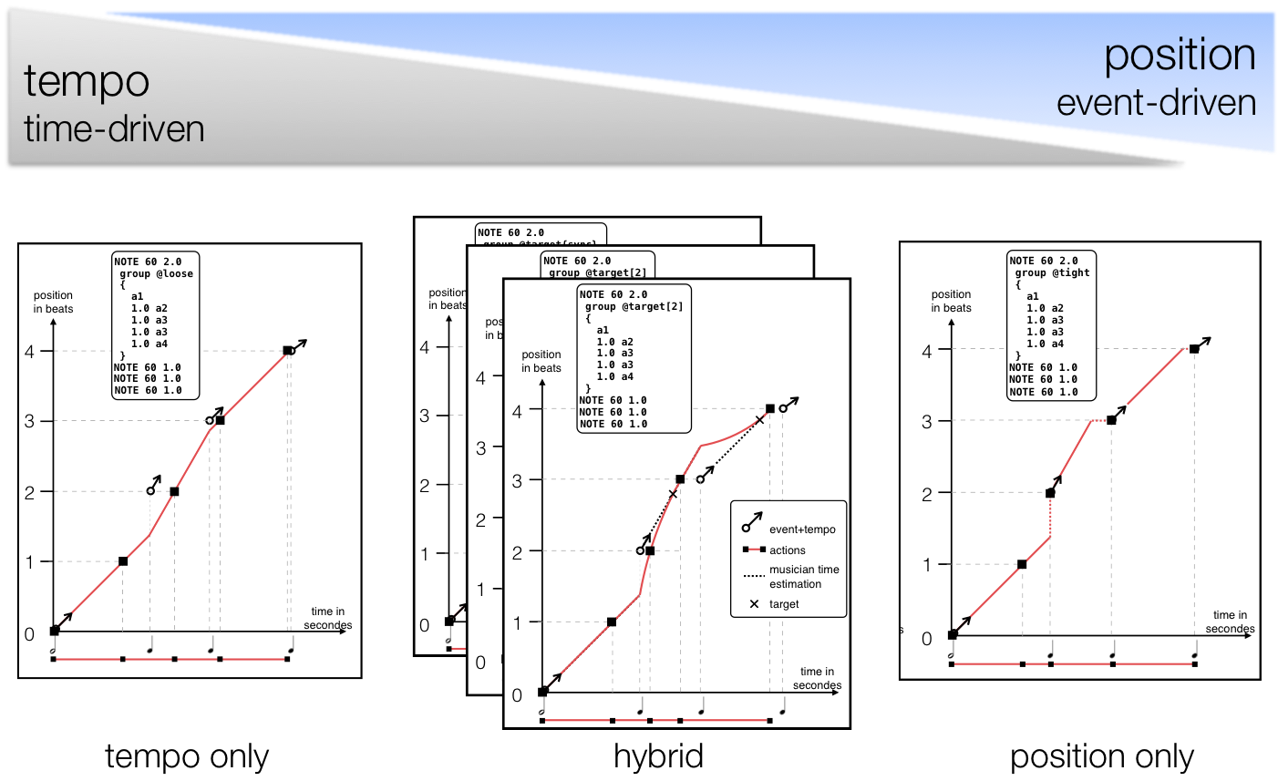
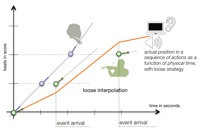
At one end of the spectrum, only the tempo information is used. This synchronization strategy is called @loose and illustrated below. With this strategy, the position of the successive events are not taken into account. Only the occurrence of the event triggering the sequence of actions is meaningful.
At the other end of the spectrum, the information of position is taken into account for each events. The tempo is only used to interpolate the change in position between two events. This is the @tight strategy. If an event happens earlier than expected, there is a jump from the current position p to the event's position p'. If an event happens later than expected, then the strategy qualifier @conservative freezes the position from time t (the date of the expected arrival) until the event's arrival at t'.
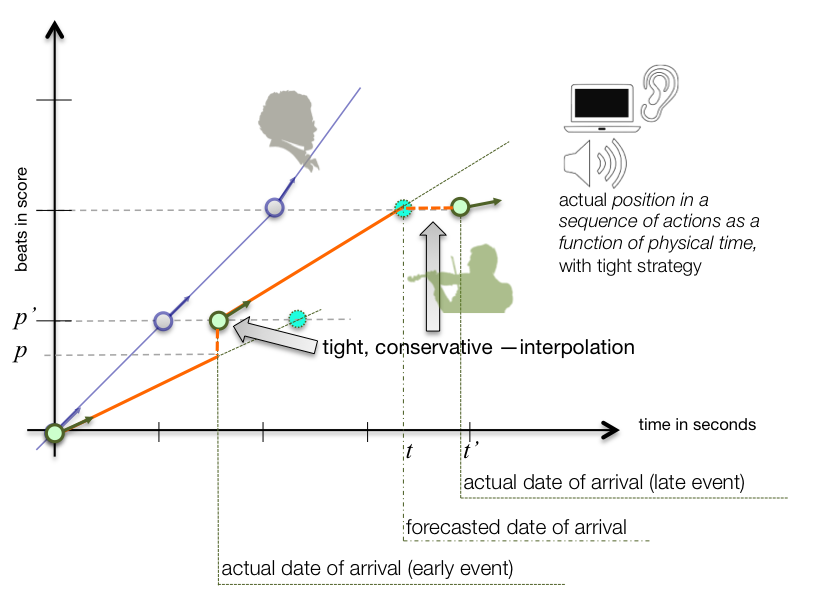
One can notice that the @loose strategy gives a smooth evolution of position with physical time, compared to the @tight synchronization strategy that may jump between position or may froze a position. The @tight strategy is relevant for actions whose progression must be synced with the onset of musical events. In between @loose and @tight behaviors, Antescofo offers strategies corresponding to an actual action time that catch up more or less smoothly with the musical events. They are all described in section synchronization strategies.
The two examples of time-time diagrams for the actual timing of actions calls for several important remarks:
-
Such a diagram can only be built in real-time, i.e. it is known only incrementally4 with the progression of the performance.
-
At an instant t, the tempo T is known because there is a method to extract the tempo information from the past audio input2. Antescofo assumes that the current tempo is known at each musical event and it is supposed to remain constant between events (in absence of specific [BPM] specification in the score).
-
The position can be a discontinuous and partial function of time.
-
The relation between the actual position and the actual tempo is non-newtonian: the actual position is not the integral of the actual tempo5.
They are indeed several ways to interpolate the positions between two events but no privileged way to choose one against the other. For instance, in the previous diagram, when an event happens later than expected, the position is frozen from the expected date of arrival t to the actual date of arrival t'. Another option, the @progressive attribute, would progress at the tempo rate, and jump back to the expected position when the event occurs (which means that the progression in the score is not monotonically increasing with physical time and makes a zig-zag).
Synchronizing with an Arbitrary Time
Our discussion focused on the specification of the actual time of electronic actions, by synchronization with a human performer. But for the Antescofo runtime, the human performer is simply a process that produces events associated with a tempo.
Such processes can be abstracted in Antescofo with a tempovar: a tempovar is a variable introduced with the @tempovar declaration. Assigning this variable corresponds to an event and a tempo is automatically derived using the algorithm used for the human performer by the listening module.
It is then possible to specify that a sequence of actions synchronized relatively to this tempovar. The only difference with the synchronization with the performer is that the performer follows an arbitrary score while a tempovar is supposed to be assigned periodically6.
A Side Note on Logical Time versus Actual Time
One conceptual advance in the field of real-time programming was the acknowledgment that time is a denotable entity, not an operational property: real-time programming language must include time in their domain of discourse.
As a consequence, modern programming languages that explicitly embed timing information within the code refer to a logical time decoupled from physical time. In this way, programs can be designed without the burden of external and operational factors, such as machine speed, portability, and timing behavior across different systems. It is then the responsibility of a compiler, an interpreter or a runtime to map this logical time with the physical time: in real-time systems, logical time aims to keep up with physical time (one logical second of logical time must take exactly one wall clock second); in non-real-time situations, logical time may run “as fast as possible” (e.g. in offline processing).
It is tempting to compare the relationships between the potential time of the score and the actual time of the electronics with the relationships between the logical time of a real-time program and the physical time of its realization. This analogy is misleading. The relationship between the potential time and the actual time of the electronic actions is not similar to the relationship between a specification and its implementation. The difference between the logical time expressed in a real-time program and the timing of its implementation accounts for the details that can be neglected in the realization. On the other hand, the potential time in the score is a partial specification. The actual time in which a sequence of actions takes place is built by a combination of three sources of information: (1) the potential time in the score, (2) the actual time of the musical events, and (3) the synchronization specifications given by the composer.
From this point of view, Antescofo differs for all other music programming languages. All music programming languages we know support only one logical time. Languages may offer several time units, like seconds, milliseconds or samples. But these unit are a priori inter-convertible (we know once and for all that 1000 ms = 1 s) and they refer to the same underlying time. The time used to schedule the electronic actions in this language is the logical time of the system.
The next section investigates the ordering of events in one instant. Then we present the synchronization strategies in depth. Finally, the last section of this chapter consider the handling of errors: as a matter of fact, our previous discussion neglected the fact that some musical events specified by the score may never happen in actual time because listening module's errors or performer's errors.
-
This property is assumed in the current version (0.9x). Future versions will consider the specification of non piece-wise constant tempo like accelerando. ↩
-
E. Large and M. Jones. The dynamics of attending: How people track time-varying events. Psychological review, 106(1):119, 1999. Other approaches may be considered. ↩↩
-
If an event e at position p happens at instant t with tempo T, then, the next event e' at position p' is predicted to happen at instant t + \frac{p' - p}{T}, i.e., we suppose that the tempo remains constant between the two events and use a linear extrapolation. ↩
-
At some point in time, the change in position as time goes, is only a non-verifiable prediction until the occurrence of an observable event which can be used to fix the position. ↩
-
The last statement derives from the penultimate: the integral of a bounded quantity cannot be discontinuous. ↩
-
Experimental extensions are considered to remove this restriction. ↩