New Interpolated Map¶
Interpolated maps are values representing a piecewise function defined by interpolation between a sequence of breakpoints.
They have been initally defined as piecewise linear functions which have been superseded by NIM (an acronym for New Interpolated Map). NIM extends the idea of interpolation between breakpoints to vectors and to a superset of the interpolation types available in the curve construct.
A NIM is an aggregate data structure that records the breakpoints of the piecewise interpolation and the interpolation type (as in a curve). A NIM is considered an extensional function like a map. It can be applied to a numerical value to return the corresponding image.
NIMs can be used as an argument of the curve construct which allows the breakpoints to be dynamically built, "playing" the function later in time. See section Curve Playing a NIM.
Continuous and Discontinuous NIM¶
NIMs can represent continuous or discontinuous functions.
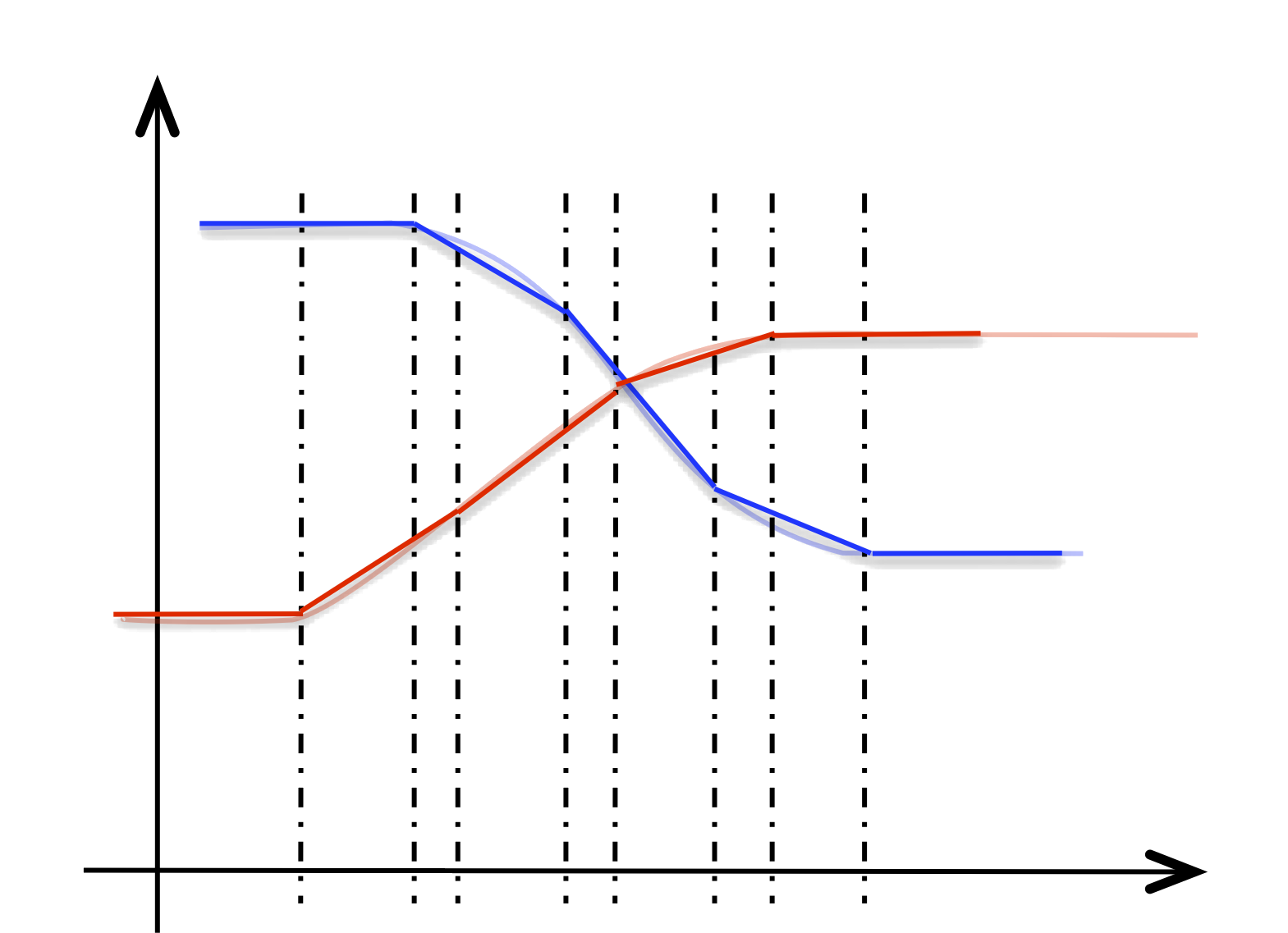
Continuous NIM are defined by an expression of the form:
         NIM { x₀ y₀, d₁ y₁  "cubic"
                    , d₂ y₂ "linear"
                    , d₃ y₃ "bounce"
                    , ...
                    , dᵢ yᵢ "tᵢ"
                    , ...
             }
which specifies a piecewise function f: between \mathtt{x}_i and \mathtt{x}_{i+1} = \mathtt{x}_i + \mathtt{d}_{i+1}, function f is an interpolation of type \mathtt{t}_{i+1} from y_i to y_{i+1}. See the following illustration:
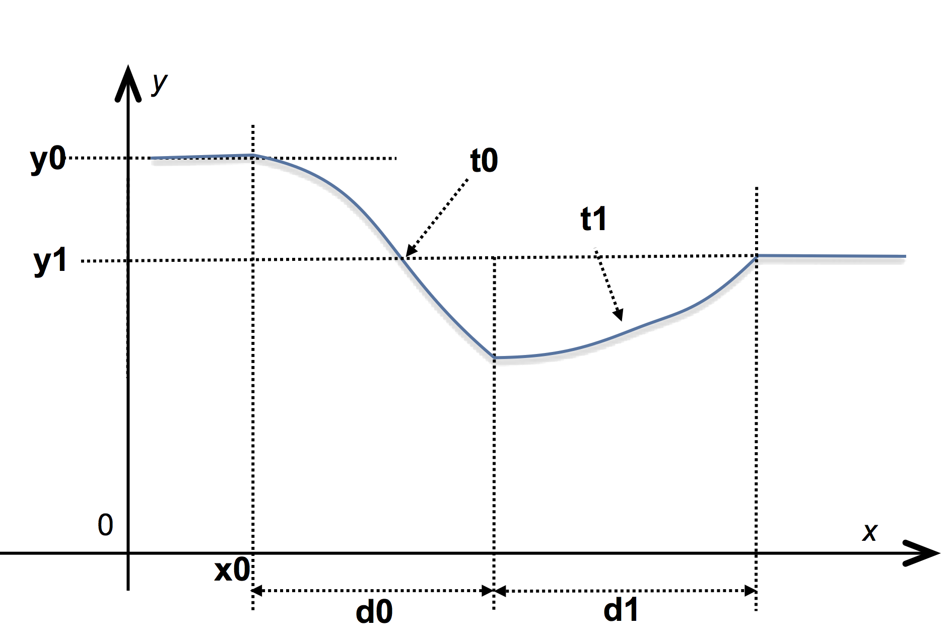
The previous definition specifies a continuous function because the value of f at the beginning of [\mathtt{x}_i, \mathtt{x}_{i+1}] is also the value of f at the end of the previous interval.
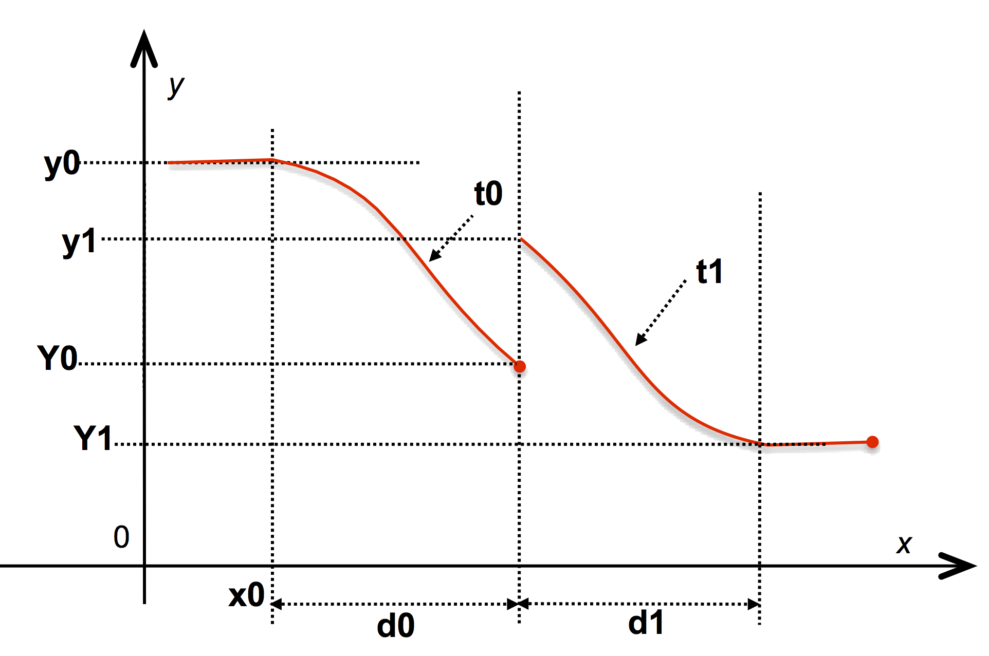
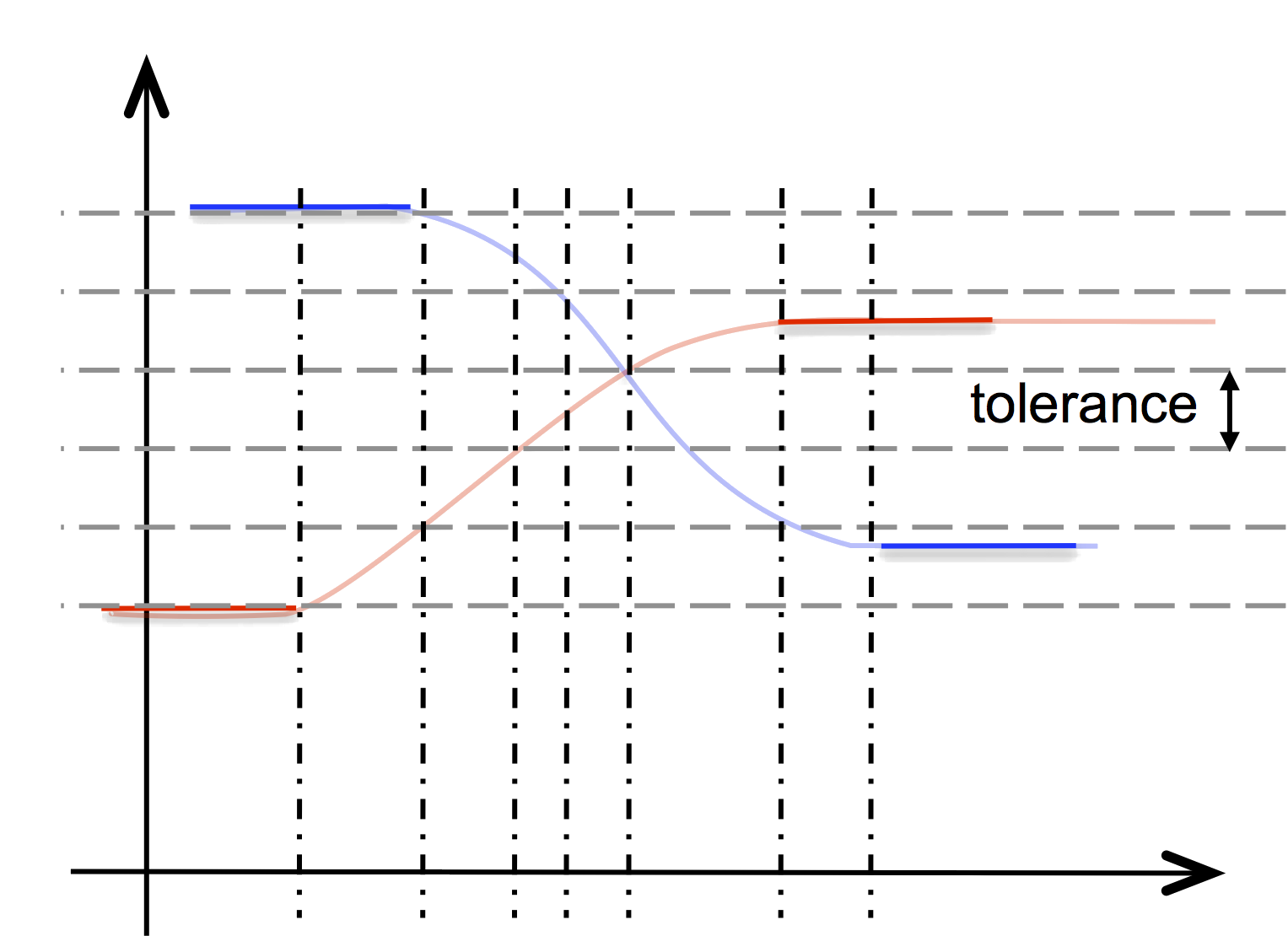
A second syntax allows one to define a discontinuous function by specifying a different value for the end of an interval and the beginning of the next one:
         NIM { x₀, y₀ d₀ Y₀  "cubic"
                 , y₁ d₁ Y₁  "linear"
                 , y₂ d₂ Y₂  "bounce"
                 , ...
             }
The definition is similar to the previous form except that on the interval [\mathtt{x}_i, \mathtt{x}_{i+1}] the function is an interpolation between \mathtt{y}_i and \mathtt{Y}_i. See illustration:
The NIM keyword is case-unsensitive and introduces an
expression. The parameters \mathtt{x}_i, \mathtt{y}_i, \mathtt{d}_i,
\mathtt{Y}_i, \mathtt{t}_i are closed expressions.
The parameters \mathtt{d}_i in a NIM expression are
relative increments on the X axis that specify the duration of the
breakpoints. It is possible to specify directly absisses using the
§ marker (remark that the marker § is also
accordingly used to specify
date-delays). For example
NIM { -1 0, §2 2, §10 10 } is equivalent to NIM { -1 0, 3 2, 8 10}
NIM { -1 0, §2 2, $10 10, 5 15 }
The use of absolute breakpoints can lead to non well-fromed nim specification, like
NIM { -1 0, §10 2, §5 10 }
wich raises an evaluation error:
Error: Nim construction: breakpoint's sequence does not progress with the absolute date '5'
Error:                   set breakpoint interval to zero
This error is non-fatal and the faulty breakpoints are set with an interval of zero.
Definition of the NIM outside the breakpoints¶
The function f is extended outside [\mathtt{x}_0, \mathtt{x}_n] such that
However, the functions @min_key and @max_key return \mathtt{x}_0 and \mathtt{x}_n respectively (these functions also perform similarly on maps: maps are functions on a discrete range while NIMs are functions on a continuous range).
Interpolation type¶
The type of the interpolation is either a constant string or an expression. In the latter case, however, the expression must be enclosed in parentheses. The names of the allowed interpolation types are the same as those of a curve (see curve interpolation methods), and the interpolation types are illustrated on these figures. Other experimental interpolation methods are currently under development.
The specification of an interpolation type is optional. When not defined, the interpolation type is assumed to be linear.
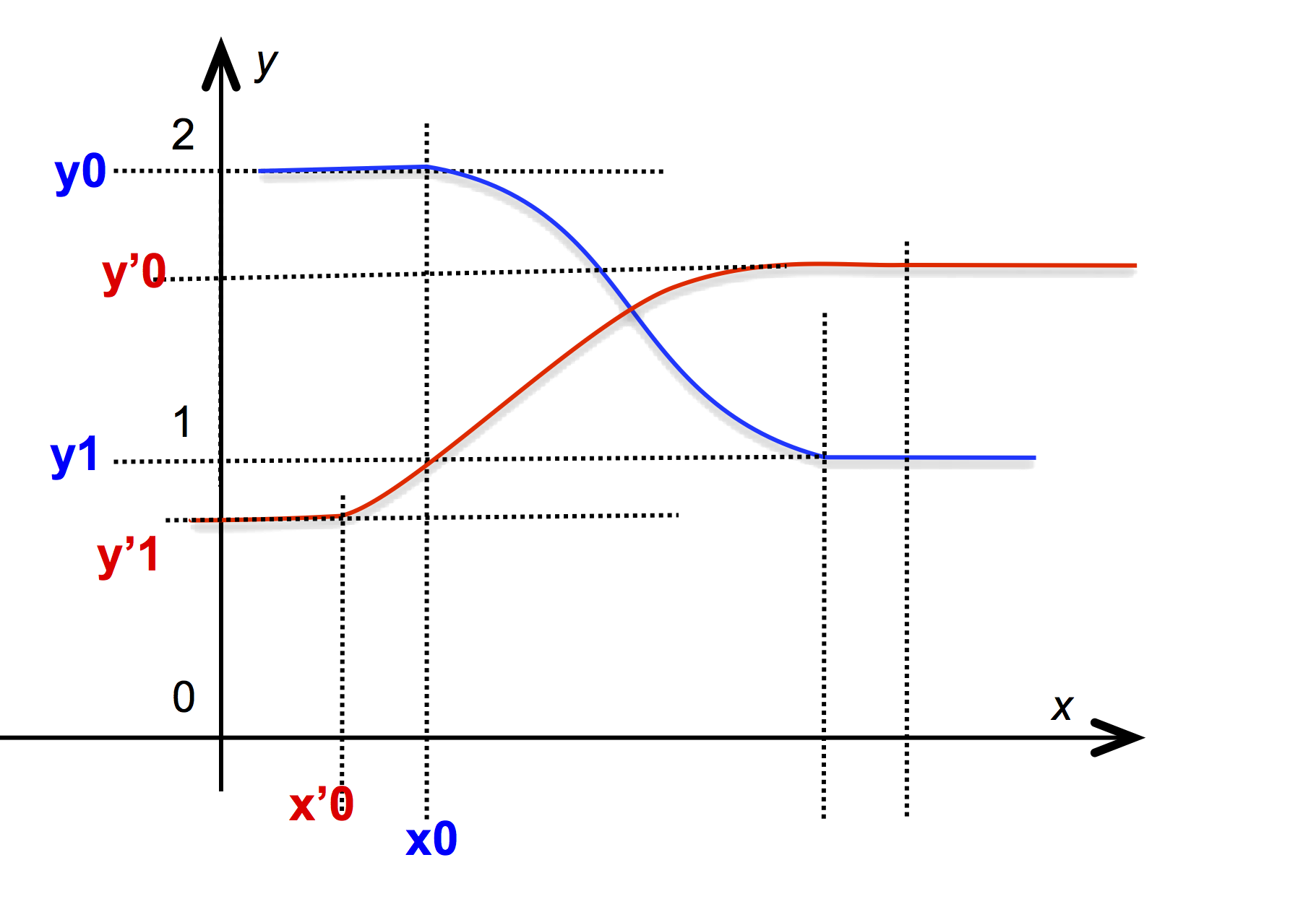
Vectorial NIM¶
The NIM construct accepts tabs as arguments: in this case, the result is a vectorial function. For example:
NIM{ [-1, 0] [0, 10], [2, 3] [1, 20] ["cubic", "linear"] }
defines a vectorial of two variables: $$ \vec{f} \binom{x_1}{x_2} = \binom{\,f_1(x_1)\,}{\,f_2(x_2)\,} $$ where f_1 is a cubic interpolation between 0 and 1 for x_1 going from -1 to -1 + 2 = 1 and f_2 is a linear interpolation between 10 and 20 for x_2 going from 0 to 0 + 3 = 3.
The NIM construction is ‟smart”: the parameters of a vectorized NIM may mix scalar s and tabs. In this case, the scalar is extended implicitly into a vector of the correct size whose elements are all equal to s. This is the case even for the specification of the interpolation type. For example:
NIM{ 0, 0, [1, 2] 10 }
defines the function \vec{f} = \binom{f_1}{f_2} where
and
A vectorized NIM is listable: it can be applied to a scalar argument. In this case, the scalar argument x is implicitly extended to a vector of the correct dimension: $$ \newcommand{\MYatop}[2]{\genfrac{}{}{0pt}{}{#1}{#2}} \vec{f}(x) = \vec{f}\binom{x}{\MYatop{\displaystyle{x}}{\displaystyle\dots}} $$
The function @dim returns the dimension of the image of a NIM, that is, 1 for a scalar NIM and n \not= 1 for a vectorized NIM, where n is the number of elements of the tab returned by the application of the NIM.
The function @size returns the number of breakpoints of the NIM (which is not equal to the dimension of the NIM). Note that a nim with zero breakpoints is the result of a bad definition.
Heterogeneous breakpoints in vectorial NIM¶
A vectorial NIM can be seen as the aggregation of several scalar NIMs.
The functions @projection and @aggregate can be used to respectively extract a scalar nim from a vectorial nim and to aggregate several (scalar or vectorial) nims of dimension d_1, \dots, d_p into a nim of dimension d_1 + \dots + d_p.
          let $nim1 := NIM{ 0 0, 1 10, 1 0 "sine_in_out" }
          let $nim2 := NIM{ -1 10, 4 0 "sine_in_out" }
          let $nim3 := @aggregate($nim1, $nim2)
This process can be used to build vectorial NIMs whose breakpoints are different, as in the specification of vectorial curves. There is no syntax to directly specify such NIMs and the function @aggregate must be used to build such NIM values that are said to have heterogeneous breakpoints. When printing such a NIM, the function @aggregate is used to list its many components:
@aggregate( NIM{0 0, 1 10 "linear",
                     1 0  "sine_in_out"},
            NIM{-1 10, 3 0 "sine_in_out"} )
The function @projection can be used to extract a component from a vectorial NIM:
@projection($nim3, 1) == $nim2 → true
Extending a NIM¶
The function @push_back can be used to add a new breakpoints to an existing NIM. They are several variations:
          @push_back(nim, d, y1)
          @push_back(nim, d, y1, type)
          @push_back(nim, y0, d, y1)
          @push_back(nim, y0, d, y1, type)
          @push_back(nim₁, nim₂)
The four first forms modify the NIM ‟in-place”. The last form builds a new NIM:
-
The first two forms extend a NIM in a continuous fashion (the value at the start of the added breakpoint is the value of the last breakpoint of the NIM).
-
The next two forms explicitly specify the starting value of the added breakpoint, enabling the specification of discontinuous function.
-
The last form extends the nim in the first argument by the breakpoint of the nim in second argument. It effectively builds the function resulting in the “concatenation” of the breakpoints.
Note that @push_back is an overloaded function: it can also be used to add (in place) an element at the end of a tab.
NIM Transformation and Smoothing¶
NIMs can be managed through Nim Related Functions @aggregate @align_breakpoints [@clone] [@compose] @concat_nim @dim @filter_max_t @filter_median_t @filter_min_t @integrate @linearize @max_key @max_val @min @min_key @min_val @projection @push_back @push_front @sample [@scale_x] [@scale_y] @simplify_lang_v @simplify_radial_distance_t @simplify_radial_distance_v @window_filter_t
See their descriptions in the library. Here, we describe the notions that appear when a NIM is restructured.
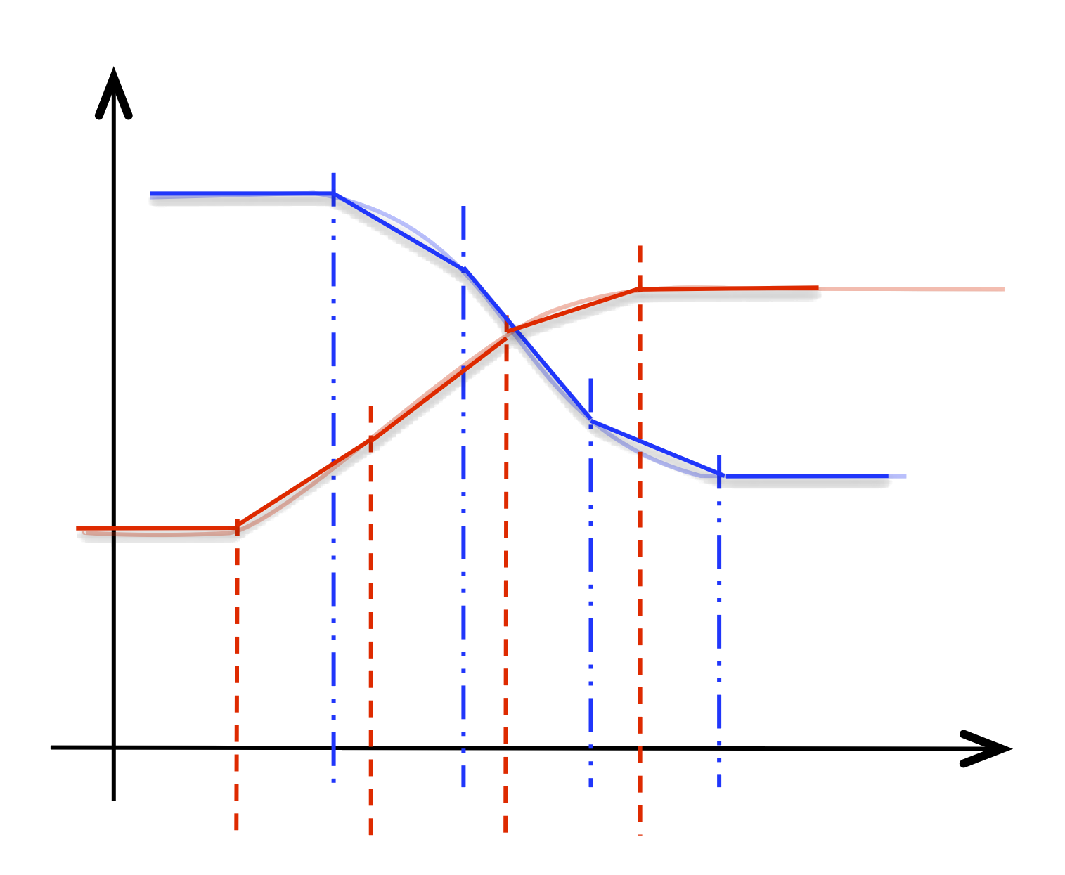
Sampling, homogeneization and linearization¶
It is possible to convert a NIM with an arbitrary interpolation type to a NIM with a linear interpolation type.
The function @sample takes a NIM nim and a number n and returns a
NIM with n breakpoints and linear interpolation type that approximates
nim. The process is illustrated in the following diagram: the NIM
$nim4 in input
@sample($nim3, 5)   →
@aggregate( nim{0 0, 0.333333 3.33333,
                     0.333333 6.66667,
                     0.333333 10,
                     0.333333 7.5,
                     0.333333 2.5,
                     0.333333 0},
            nim{-1 10, 0.5 9.33013,
                       0.5 7.5,
                       0.5 5,
                       0.5 2.5,
                       0.5 0.669873,
                       0.5 0}  )
As can be seen, in the case of a vectorial NIM with heterogeneous components, the approximation is done component by component and the result has heterogeneous breakpoints.
The function @align_breakpoints can be used on a NIM with linear interpolation type to obtain an equivalent NIM with homogeneous breakpoints:
let $nim4 := @sample($nim3, 5)
will compute a NIM with a heterogeneous breakpoint printed as
@align_breakpoints($nim4)   →
NIM { [-1, -1],
      [0, 10] [0.5, 0.5] [0, 10]
      [0, 9.33013] [0.5, 0.5] [0, 9.33013]
       ; ...
      [0, 0] [0.333333, 0.333333] [0, 0] }
The function @sample samples its NIM argument homogeneously (component
by component). This is not always satisfactory because the variation of
the NIM can differ greatly between two intervals. The function
@linearize(nim, tol) uses an adaptive sampling step to
linearize nim, to align the breakpoints and to achieve an
approximation within a given tolerance tol.
@linearize($nim3)   →
NIM { [-1, -1],
      [0, 10] [0.609946, 0.609946] [0, 9.01426],
      [0, 9.01426] [0.270743, 0.270743] [0, 8.02012],
      ; ...
      [0.563462, 0.0636838] [0.152573, 0.152573] [0, 0] }
The application of the @linearize function can be time consuming and care must be taken so as not to perturb the real-time computations, e.g., by precomputing a linearization (see @eval_when_load clause and function @loadvalue).
NIM simplification¶
NIMs can be used to record a temporal series of data arriving (through time) from the environment, using setvar or OSC messages. It is then often useful to simplify the NIM, in order to have a more compact representation. The underlying idea is that the NIM approximates a curve known by a series of points, the breakpoints of the NIM, and that this curve can be approximated by fewer points. The simplified NIM consists of a subset of the breakpoints that defined the original.
Several functions can be used to achieve a reduction of the number of breakpoints of a NIM with linear interpolation.
All the simplification functions apply to scalar as well as vectorial NIMs, but consider only the ”x-coordinate” given by the breakpoints of the first component2. In case of a vectorial NIM with heterogeneous breakpoints, this can be a drawback. In this case, an equivalent NIM with homogeneous breakpoints can be first built using the @align_breakpoints function.
The three following functions are inspired from polyline simplification functions developed in computer graphics1:
-
@simplify_radial_distance_t
(nim, d)simplies each component of the NIM independently by reducing successive breakpoints that are clustered too closely to a single breakpoint. Because the simplification works on each component independantly, a breakpoint in this context is simply a point (x, y) in the plane. The simplification process starts from the first breakpoint and is iterated until it reaches the final breakpoints. The first and the last breakpoints are always part of the simplification. All consecutive breakpoints that fall within a distance from a kept breakpoints are removed. The first encountered breakpoints that lies further away than is kept. -
@simplify_radial_distance_v
(nim, d): this simplification function is similar to the previous one but instead of working on each component independently, the vectorial nature of the nim is taken into account and the “x-coordinate” is ignored. The NIM is seen as a sequence of points, the image of the NIM at coordinates given by the x part of the breakpoint of the first component. It is this series of points that is simplified to build the new NIM. The distance is thus taken in a n-dimensional space, where n is the dimension of the NIM. -
@simplify_lang_v
(nim, tol, d): this simplification function follow the same approach as the previous one and consider a sequence of points in a n-dimensional space, where n is the dimension of the nim and the points are given by the image of the breakpoints of the first component. Then, a Lang simplification algorithm is applied to reduce the number of points. The remaining points are used to build the simplified nim.The Lang simplification algorithm defines a fixed size search-interval. The first and last points of that interval form a segment. This segment is used to calculate the perpendicular distance to each intermediate point. If any calculated distance is larger than the specified tolerance , the interval will be shrunk by excluding its last point. This process will continue until all calculated distances fall below the specified tolerance, or when there are no more intermediate points. All intermediate points are removed and a new search interval is defined starting at the last point from the old interval.
The effect of these simplification functions on a nim can be observed using the function @size which returns, for a nim, its number of breakpoints.
Smoothing and Transformation¶
The functions described here work independently on each component of a nim. They see each component as a sequence of points y (the image of the nim) that are smoothed in various way. The resulting points are used to build a new nim with linear interpolation type. The number of breakpoints is preserved, as well as their x-coordinate. Only the y-part of the breakpoint (the image) is affected.
-
@filter_median_t
(nim, n)smoother the y by replacing every image by the median in its range-n neighborhood. Notice that the median is taken in a sequence of 2 n + 1 values. The first n points and the last n points are left untouched. -
@filter_min_t
(nim, n)filters the y by replacing every image by the minimum value in a sequence of length 2 n + 1 centered on y. The first n points and the last n points are left untouched. -
@filter_max_t
(nim, n)filters the y by replacing every image by the maximum value in a sequence of length 2 n + 1 centered on y. The first n points and the last n points are left untouched. -
@window_filter_t
(nim, coef, pos)replaces every y by the scalar product ofcoef(a tab) with a sequence of n values, where n is the size ofcoefandposis the position in this window of the current y (numbering starts with 0). The firstposvalues and the last $n - $posvalues are left untouched.For example,
@window_filter_t(nim, [2], 0)builds a NIM by scaling the image of by 2.@window_filter_t(nim,[0.1, 0.2, 0.5, 0.2, 0.1], 2)is a moving weighted average with symmetric weights around y.
-
The following references gives technical details on polyline simplification. Description and evaluation of several algorithms in a cartographic context are given in this paper. The Ramer–Douglas–Peucker algorithm follows an idea similar to the Lang algorithm used by @simplify_lang_v but the shrinking of the current interval is dichotomous. This project provides an implementation of the main algorithms is in C++. ↩
-
If the recorded value is a time series, then the x-coordinate corresponds to time and the NIM will be homogeneous as it is incrementally built using the function @push_back. The only way to build a non-homogeneous nim is to use the function @aggregate. ↩