Differential Curve (experimental)
Differential curves are curves with an underlying function defined by a set of ordinary differential equations (ODEs) and some switching points between them, instead of an explicitly piecewise defined functions.
The uses of a differential curve are the same as an ordinary curve: only the specification of the sampled function differs. Differential equations are used to define the sampled function by a property instead of giving an explicit formulation and zero-crossing point (see below) define implicit breakpoints.
Differential curves are still experimental and requires a dedicated
object or a dedicated standalone. One may test if this feature is
available by testing if the function @ode_solve
exists. For instance, you can developp code using differential curve in
a conditional code region:
          #if @ode_solve
          ; ... code using ode curves
          #endif
Introduction
A differential curve is a device used for the numerical resolution of an initial value problem posed in explicit form, as:
y' = f_E(t, y) + f_I(t, y)
y(t_0) = y_0
the independant variable t is the time and the dependant variables are given by y \in \mathbb{R}^n. The dimension of the system is the integer n. The previous formulation can be seen as a set of n coupled differential equations defining the y_i elements of the vector y.
By explicit form, we mean that the specification of y' is given by an expression which does not imply y'. The equation considered is also first-order meaning that only the derivative of y appears in the equation. However, such systems are extended to higher orders by treating the derivatives in the same way as additional independent function, e.g. extending the vector y to represent explicitly y_i'' for some i by an additional element y_{n+1}.
The notation y' denotes the derivative \frac{dy}{dt} of y. The value y_0, called the initial condition, is the value of the unknown function y(t) at the time t_0 at which the differential curve is launched. The functions f_E and f_I are the evolution functions:
-
f_E(t, y) constains the “slow” time scale components of the system. This will be integrated using explicit methods;
-
f_I(t, y) contains the “fast” time scale components of the system 1. This will be integrated using implicit methods that are more stable and robust to numerical errors.
Either of these operators may be disabled, allowing for fully explicit, fully implicit, or combination implicit-explicit time integration. The terms “explicit” and “implicit” used here qualify the numerical schema used by the solver for the resolution, not the form of the ODEs, which are always in explicit form2. More information on this distinction is given below.
The differential curve computes a numerical approximation of the unknown
function y(t) as a periodic sampling of the solution y specified by
the @grain attribute of the curve. At each sampling
points, the actions specified through attribute @action
are performed. If there is no such action, the sampling points are still
computed (as for an ordinary curve). Notice that the @grain has nothing to do with the step used by numerical solver used to
compute the values of y. This step is controled internaly and
dynamically adapted to achieve the numerical precision required by the
resolution (see sect. Tolerance and error
control below).
Actions can also be triggered at other time-points than the sampling points. These time points t_z are defined implicitly by an equation representing a threshold crossing. These points are called zero-crossing points. At some of these points, called switching points, the current state y(t_z) of the system or the system's evolution functions f_I and f_E, can be changed. So, a differential curve effectively combine continuous-time with discrete-event behavior, mathematically representing hybrid dynamic systems.
Antescofo relies on the ARKode numerical solver part of the SUNDIALS SUite of Nonlinear and DIfferential/ALgebraic Equation Solvers for the numerical resolution and the detection of zero-crossing points.
System specification
Syntax
The syntax of a differential curve is the syntax of an ordinary curve except for the specfication of its body.
The body of a differential curve is composed of three sections: the specifciation of the initial system (a state and a differential equation), a set of parameters, and the specification of zero-crossing points and their associated behavior.
Initial system
The initial state is defined by an expression which evaluates into a vector:
and by an equation which defines the evolution function:
The variable $var that appears in the left hand side and
in the right hand side of the equation must be the same as the variable
in the left hand side of the initial condition. At any moment after the
start of teh curve, this variable will refer to the current state of the
system. This state is a tab of float. The size n of this tab is
the dimension of the system.
The evolution function @f is the name of a user-defined
function. The prefix explicit:: or implicit:: specifies if the function belongs to the slow (explicit) or
fast (implicit) components. If there is no prefix, the function is
assumed to be explicit. They can be at most one implicit and one
explicit component. If the two components are defined, the two terms are
added.
The arguments between square brackets remind the arguments of the
function, but there is few freedom in the declaration: the time variable
is either $NOW or $RNOW, meaning that the
idependant variable is the absolute time or the relative time. The
second argument must the variable that represents the current state of the
system.
Signature of the evolution function
For efficiency reason, the evolution function is not a binary function
but a ternary one. Function @f takes 3 arguments:
-
the first argument refers to the temporal variable t
-
the second argument refers to the state y of the system
-
the third argument refers to the derivative y'.
The value of the first two arguments t (a float) and y (a tab of
floats) represent the state y(t) at some point t. These arguments
are given to the evolution function which must update the elements of
its last arguments (which is also a tab of float). Tab y and y' have
the same dimension. The evolution function must returnsan integer:
0 if everything goes fine, and a non zero value if there
is an error.
Beware: Function @f is called during the numerical
resolution at arbitrary points. The numerical method makes adaptive
steps to minimize computations and error control requires additional
evaluation of the evolution function. In addition, Antescofo
anticipates some computations. So, the value of the temporal variable
does not reflect the actual time when the evolution function is called.
The numerical computation are done asynchronously with respect to the
actual time. Nevertheless, when the @action of the curve
is performed, the variable $var specified by the equation
refers to the state of the system corresponding to the current time.
A spring mass system
Consider a mass $m$ hanging at the end of a spring. Hooke's law gives the relationship of the force exerted by the spring when the spring is compressed or stretched a certain length: $F = -k x$ where $F$ is the the restoring force the spring exerts, $k$ is the spring constant, and $x$ is the displacement of the mass with respect to the equilibrium position. The negative sign indicates that the force the spring exerts is in the opposite direction from its displacement.
So the system state $y$ can be represented by the two quantities: $x$ the position of the mass and its speed $x'$. Using the square brackets to denote a vector, we have $y = [x, x']$ So $y' = [x', x'']$.

The fundamental law of mechanics states that m x'' = F, so y' = [y[1], - \frac{k}{m} \, y[0]]. The computation of the successive positions of the mass can then be implemented by the following antescofo program (we assume k/m = 1):
        @fun_def @f($t, $y, $ydot)
        {
             $ydot[0] := $y[1]
             $ydot[1] := -$y[0]
             return 0
        }

        curve
        @action { print $y }
        @grain 0.05 s
        {
              $y = [0, -1]
              $y' = @f[$NOW, $y]
        }
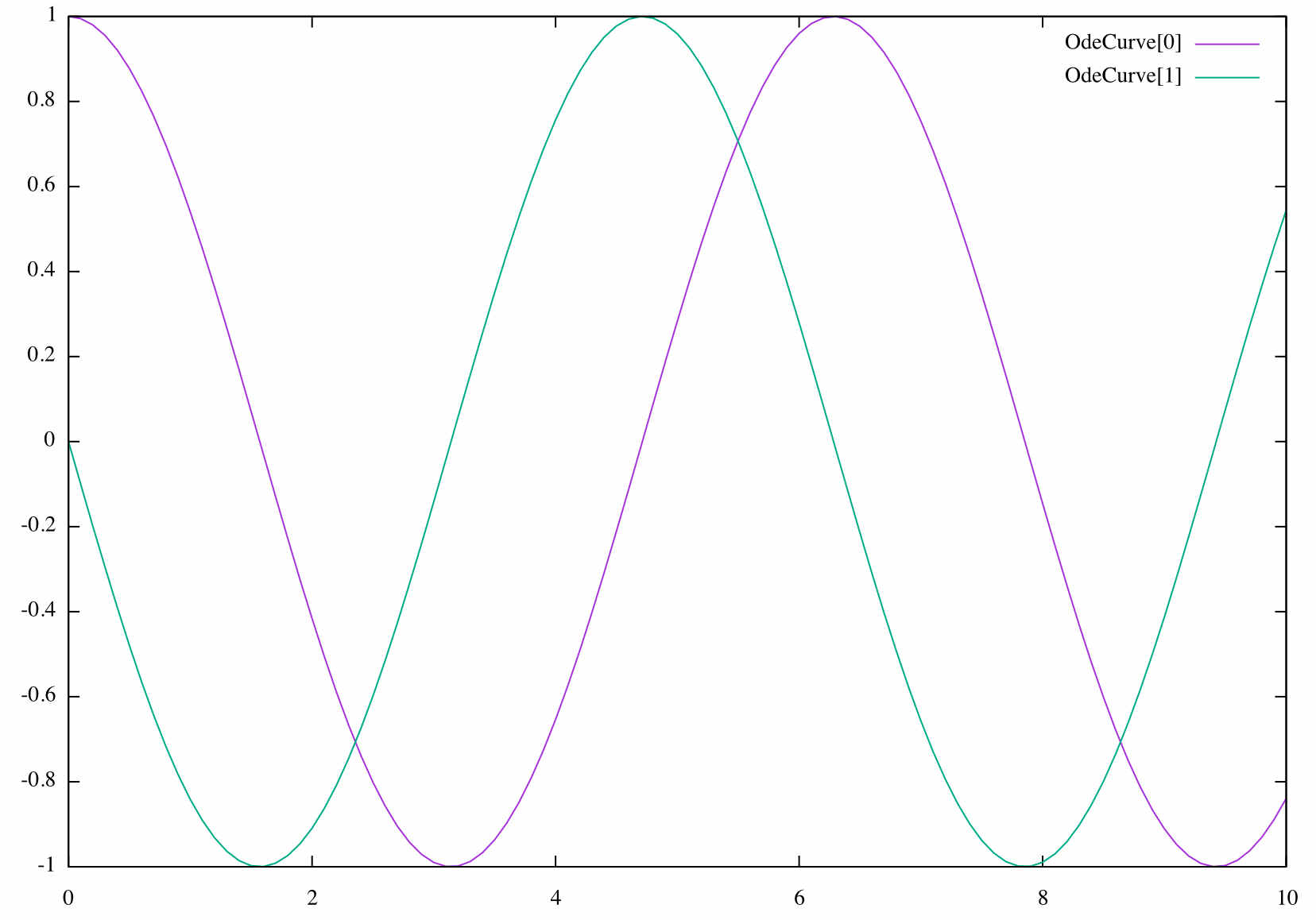
The initial state represents a system where the mass is at the rest
point with a speed of -1. The behavior of the masss if that of an
harmonic oscillator. The following diagram plot the values of
$y in time. The position (in blue) is extremal with a
speed (in green) of zero, and vice-versa.
Zero-crossing points
The numerical resolution is augmented to include a rootfinding feature. This means that, while integrating the differential equation, the numerical solver can also find the roots of a set of user-defined functions g(t, y) that depend on the independant variable t and the solution vector y.
What is really detected is the change of sign of g(t, y(t)) and the rootfinding device is able to detect the direction of the crossing. But if a root is of even multiplicities (no sign change), it will probably be missed by the solver. This is why we call “zero-crossing points” the roots found by the solver.
When a zero crossing point is detected, four kind of actions can be performed:
-
launching arbitrary antescofo actions,
-
changing the current system's state,
-
changing the evolution function,
-
changing both the current system's state and the evolution function.
A curve may defines an arbitrary number of zero-crossing points. The zero-crossing points on which the system's state or the evolution function change, are called switching points.
Zero-crossing points detection
Zero-crossing points are specified in the body of the curve using a
special form of whenever
The body of the whenever depends on the action undertaken on the
detection of a zero-crossing point. The symbol between expressions
expr₁ and expr₂ specifies the direction of
the crossing:
-
expr₁ =>= expr₂detects when the value ofexpr₁is greater than the thresholdexpr₂and becomes lower; -
expr₁ =<= expr₂detects when the value ofexpr₁is below the thresholdexpr₂and becomes greater; and -
expr₁ === expr₂detects when the value ofexpr₁pass through the thresholdexpr₂in any direction.
The relationships between the function g mentionned above and the
expression expressions expr₁ and expr₂ is
simple : g(t, y) = expr₁ - expr₂.
Launching actions on a zero-crossing point
Actions can be launched at each sampling point: sampling points are
defined with the @grain attribute and the associated
action with the @action attribute of the curve.
It is possible to launch actions each time a zero-crossing point is
detected by declaring these actions in the body of the whenever clause of the differential curve. We illustrate this
construction with the modeling of a falling ball.
A falling ball
The state y = [z, z'] of the system is defined by the vertical
position z and the speed z' of the ball. Gravity exerts a constant
force on the ball. With the choice of the appropriate unit, we have:
y'[0] = y[1] and y'[1] = -1. And we want to detect when the ball
reach the floor, i.e., when z =>= 0. Thus:
          @fun_def g($t, $y, $ydot)
          {
                $ydot[0] = $y[1]
                $ydot[1] = -1
                return 0
          }

          curve
          @grain := 0.1
          {
               $y := [1, 0]
               $y' := @g[$NOW, $y]

               whenever $y[0] =>= 0
               { print floor reached at $NOW }
          }
Running the previous program print on the console:
floor reached at 1.41421
Switching points
We want to extend the previous example to model a bouncing ball: when the ball hits the floor, the speed is instantaneously reversed. The evolution function remains the same.
To model this behavior, we add an additional zero crossing point, similar as the previous one, but the associated action is to switch the current state to the new one:
          @fun_def switch_speed($t, $y, $y_new)
          {
                $y_new[0] := $y[0]
                $y_new[1] := - $y[1]
                return 0
          }

          curve
          @grain := 0.1
          {
               $y := [1, 0]
               $y' := @g[$NOW, $y]

               whenever $y[0] =>= 0
               { print floor reached at $NOW }

               whenever $y[0] =>= 0
               { $y =  @switch_speed[$NOW, $y] }
          }
Notice the specification of the new state: it is given by a function that has the same signature of the evolution function. But in the case of a switching point, the last arguments represents the new state (this interface makes possible to manage efficiently all memory allocation).
The program execution for 10 seconds gives:
        floor reached at 1.41421
        floor reached at 1.41421
        floor reached at 4.24264
        floor reached at 4.24264
        floor reached at 7.07107
        floor reached at 7.07107
        floor reached at 9.89949
        floor reached at 9.89949
This is not what is expected: crossing points are detected two times on apparently the same t despite the detection is done in only one direction.
The problem is that our specification of the behavior at the switching point is not robust. The correct specification of the behavior at a switching point is usually subtle and requires some care to avoid two problems.
The first problem is that the numerical resolution is an
approximation. So the value of $y[0] is not exactly 0,
but in a very close neighborhood. This neighborhood depends of the error
tolerance we fix to the solver (see below).
The second problem is the discontinuity of the speed at the switching point (strictly negative before and strictly positive after). A small error in the time variable may leads to a great difference in the derivative which induce a big change in the position.
So it is better to impose the knowledge we have on the switching point:
the position is 0 and at this point, the speed is positive. So we do not
assume that $y[0] is zero, nor than at this point, the
speed $y[1] is negative. This leads to a more robust
specification of the state changes:
          @fun_def switch_speed($t, $y, $y_new)
          {
                $y_new[0] := 0
                $y_new[1] := @abs($y[1])
                return 0
          }
With this function, running the program for 10 seconds gives:
        floor reached at 1.41421
        floor reached at 4.24264
        floor reached at 7.07107
        floor reached at 9.89949
which what is expected.
Changing the current state
Suppose now that each time the ball hits the floor, it also looses some energy, resulting in a loss of 30% of its speed. The specification of new state becomes
          @fun_def switch_speed($t, $y, $y_new)
          {
                $y_new[0] := 0
                $y_new[1] := 0.7 * @abs($y[1])
                return 0
          }
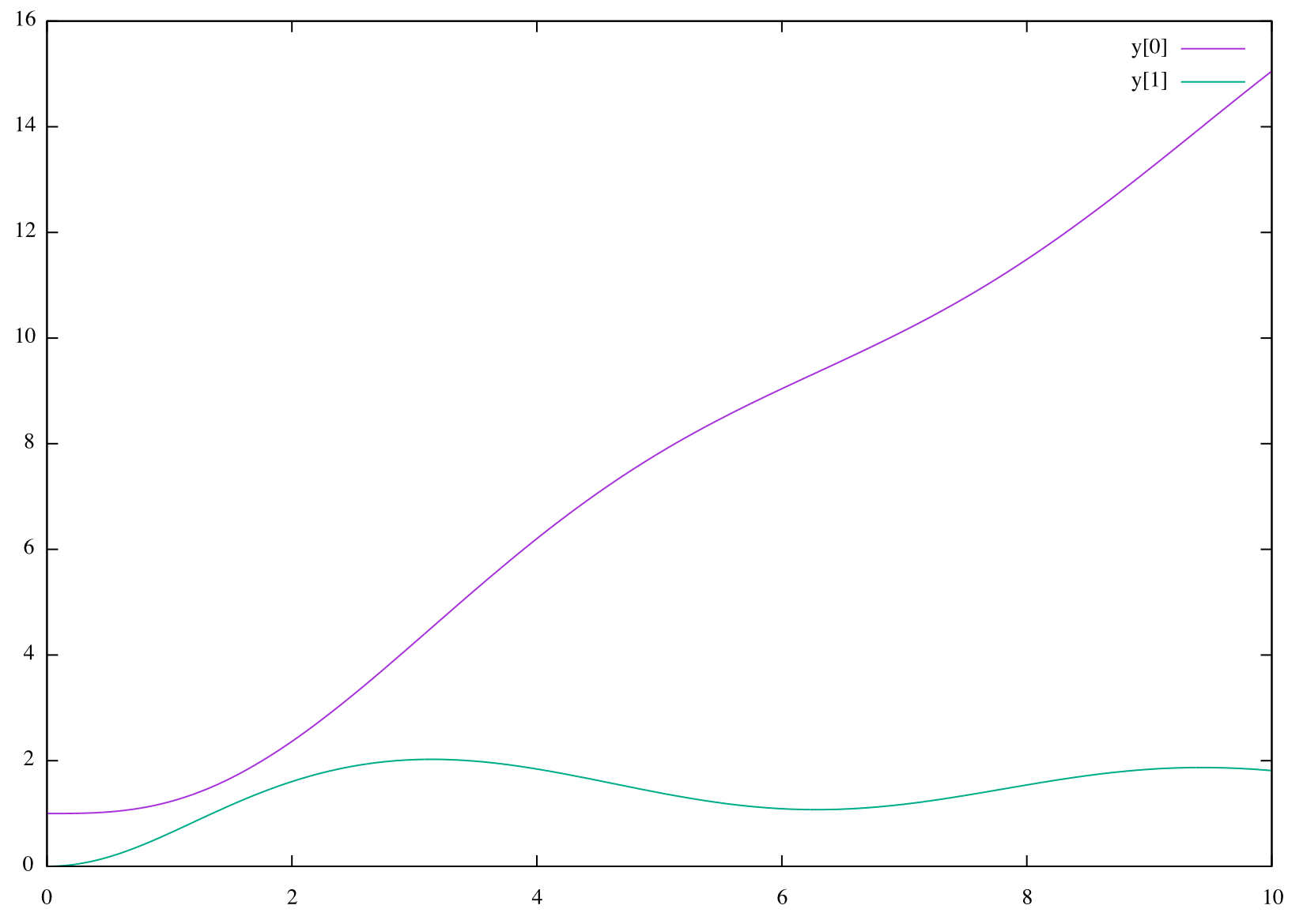
The result is plotted in the figure below:
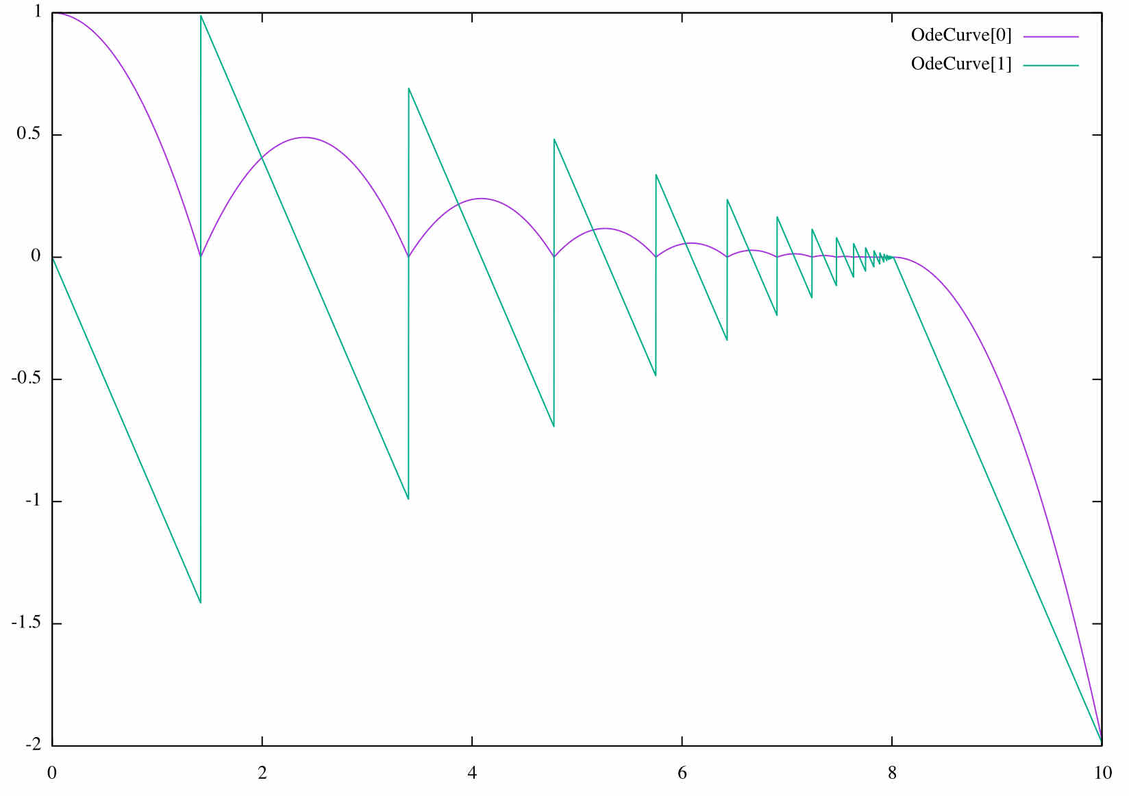
Again, we have a problem of instability. When the speed becomes very small, the numerical precision is not enough and the ball goes under the floor due to a numerical approximation, at which point the ball continue to fall attracted by the gravity.
The solution is to change the evolution function to stop the oscillations of the ball when its speed is small enough when the position is around 0. When such a condition is detected, we change the evolution function to suppress the gravity:
@fun_def zero($t, $y, $y_new)
{
$y_new[0] := 0
$y_new[1] := 0
return 0
}
curve
@grain := 0.001
{
$y = [1, 0]
$y' = @g[$NOW, $y]
whenever $y[0] =>= 0
{ print floor reached at $NOW }
whenever $y[0] =>= 0
{ $y = @switch_speed[$NOW, $y] }
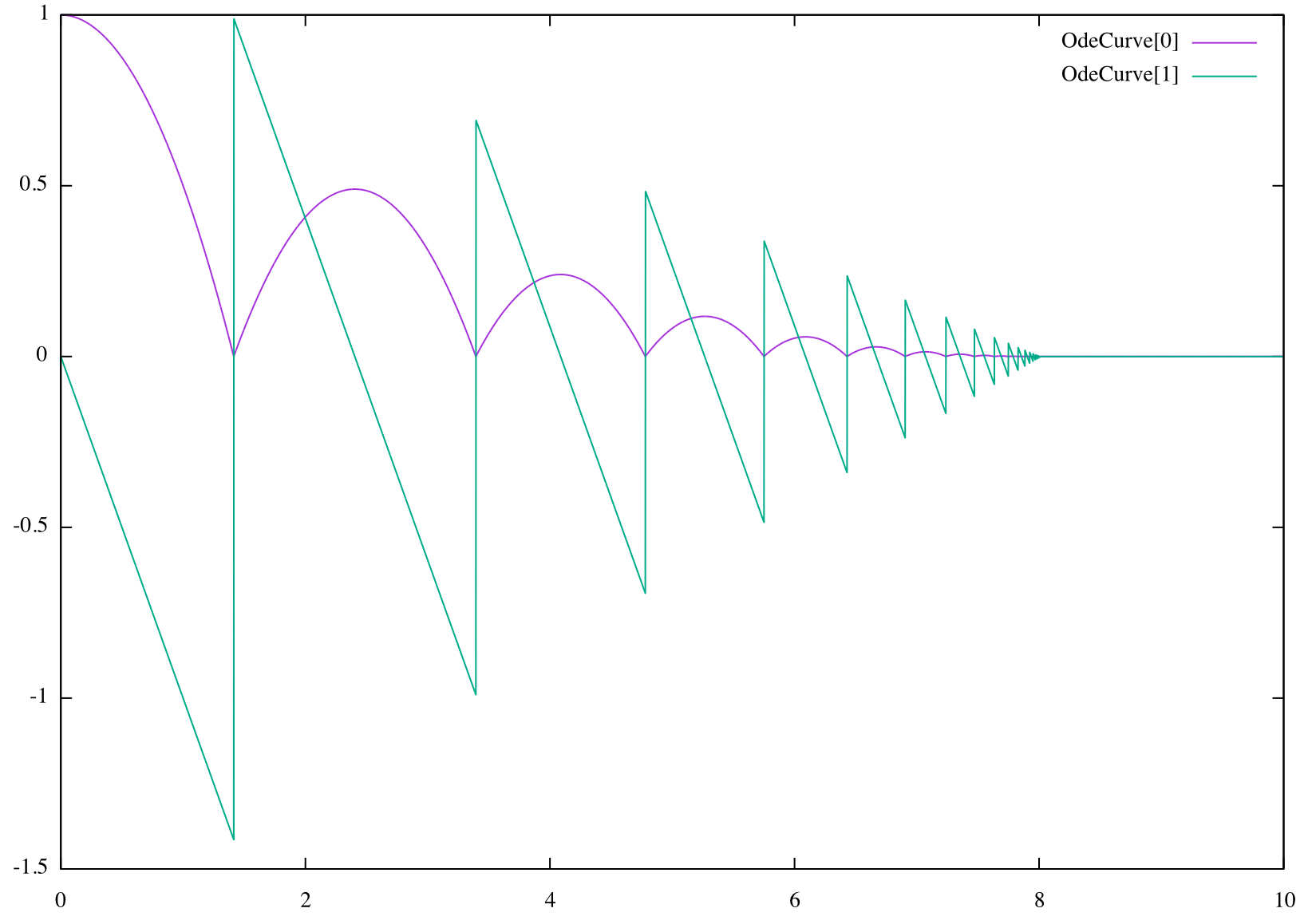
whenever @abs($y[1]) + @abs($y[0]) == 0.0001 {
$y' = @zero[$NOW, $y]
$y = @zero[$NOW, $y]
}
}
Here, the switching point used to change the state and the evolution function is specified as |z| + |z'| crossing 10^{-4}. At this point, the position and the speed is set to zero, and the evolution function keeps theses value at zero.
Stiff evolution function
The numerical solver used by Antescofo relies on more stable methods to compute the solution of stiff components. These more stable methods come often with a higher computational price3, this is why, by default, explicit methods are used.
The interested will find in the ARKode documentation a detailed
Switching between explicit or implicit methods is controlled by the prefix of the evolution function. We illustrate this feature on the Brusselator, a theoretical model for a type of autocatalytic reaction (example taken verbatim from the arkode solver documentation. The ODE system has 3 components, y = [u, v, w] satisfying:
u' = a - (w+1)u + v u^2
v' = w u - v^2
w' = \frac{b - w}{\epsilon} - w u
with the initial values and constants: u_0=1.2, v_0=3.1, w_0=3 and a=1, b=3.5, \epsilon=5.10^{−6}. With these parameters, there are rapid evolution at the beginning, and around t = 6.5.
We solve this system with two curve: C1 defines the
evolution function as fully explicit and C2 defines
the evolution function as fully implicit.
@macro_def @A   { 1.2 }
@macro_def @B   { 2.5 }
@macro_def @EPS { 1.e-5 }

@fun_def @f($t, $y, $ydot)  // y = [u, v, w]
{
     $ydot[0] := @A - ($y[2] + 1.0)*$y[0] + $y[1] * $y[0]* $y[0]
     $ydot[1] := $y[2] * $y[0] - $y[1] * $y[0] * $y[0]
     $ydot[2] := (@B - $y[2])/@EPS - $y[2] * $y[0]

     return 0
}

curve C1
@grain := 0.01 s
{
     $z = [3.9, 1.1, 2.8]
     $z' = @f[$NOW, $z]

     tolR = 1.e-8
     tolA = 1.e-8
}

curve C2
@grain := 0.01 s
{
     $z = [3.9, 1.1, 2.8]
     $z' = implicit::@f[$NOW, $z]

     tolR = 1.e-8
     tolA = 1.e-8
}
Macros are used to specify the constants in the evolution function
(using variables is not possible because evolution functions are
compiled, cf. below). The pair name = val that appears
after the specification of the evolution function and of the initial
state are parameters of the solver. They specify an absolute and
relative tolerance of 10^{-8} used at various level (error estimation,
integration, etc.). Parameters are explained in the next section.
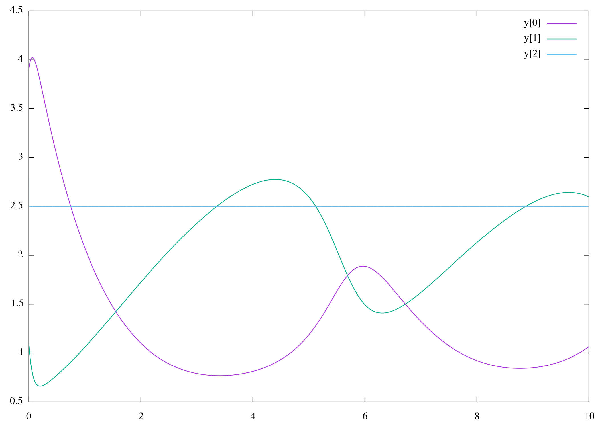
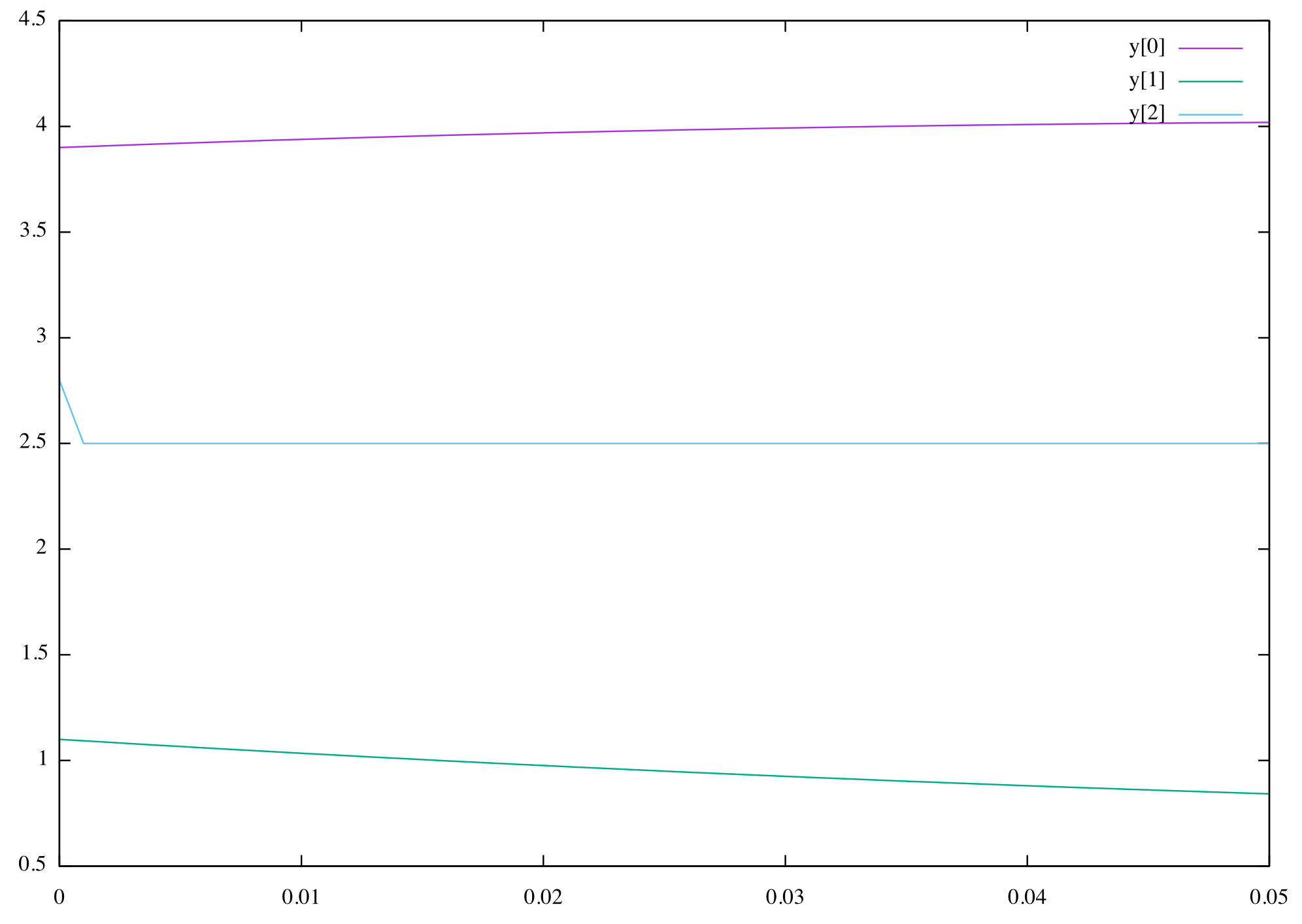
The plot at the left shows the evolution of u (in blue), v (in green) and w (pale blue). All three components exhibit a rapid transient change during the first 0.2 time units, followed by a slow and smooth evolution. The abrupt change in w is visible in the zoom at the right (open the figure in another window to see a larger view).
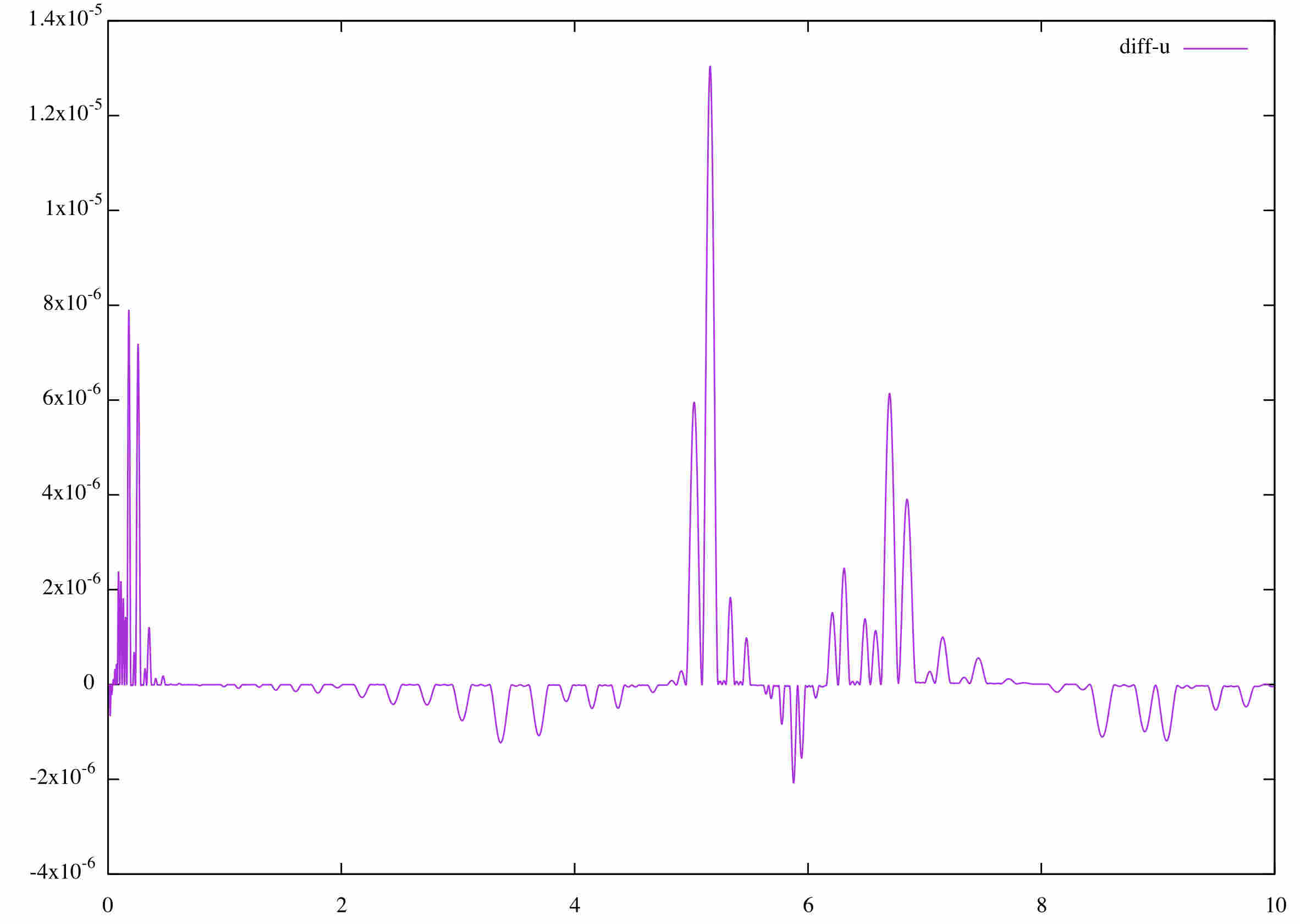
The difference between the two methods is shown on the following plot. Difference up to 10^{-5} appears, despite the fact that the error is set to 10^{-8}.
It is also possible to split the evolution function into stiff f_I and non-stiff f_E components:
f_I(t, y) = [0, 0, \frac{b - w}{\epsilon}]
f_E(t, y) = [a - (w+1)u + v u^2, w u - v^2, -w u]
which leads to the following curve:
@fun_def @fE($t, $y, $ydot)
{
     $ydot[0] := @A - ($y[2] + 1.0)*$y[0] + $y[1] * $y[0]* $y[0]
     $ydot[1] := $y[2] * $y[0] - $y[1] * $y[0] * $y[0]
     $ydot[2] := (@B - $y[2])/@EPS

     return 0
}

@fun_def @fI($t, $y, $ydot)
{
     $ydot[0] := 0.
     $ydot[1] := 0.
     $ydot[2] := - $y[2] * $y[0]

     return 0
}

curve C3
@grain := 0.01 s
{
     $x = [3.9, 1.1, 2.8] // [ 1.2, 3.1, 3.0]
     $x' = explicit::@fE[$NOW, $x] + implicit::@fI[$NOW, $x]

     update_new = true
     tolR = 1.e-8
     tolA = 1.e-8
     order = 5
}
Parameters
The behavior of differential curves can be controlled through a set of
parameters. The parameters values are specified by a list of
name = value pairs, afters the specification of the
initial state and of the evolution function, and before teh
specification of the crossing points. Some parameters are related to the
Antescofo management of the solver, and some impact directly the
behavior of the solver.
Antescofo Parameters
State dimension dim
To optimize the management of the memory, Antescofo requires to known in advance the dimension of the system. Currently, this dimension is fixed across switching points.
Knowing “in advance” means at parse time, before the program
execution. Sometimes it is possible to infer statically the dimension
from the expression used to specify the initialization state, without
evaluating it. If not, one must specify explicitly the dimension of the
system using the dim keyword.
State memory management pure
The value of the dependent variable y, the state of the system, is a vector computed by the solver. internally, to spare memory allocation, this vector is updated in-place and not build in the evolution function or in the function used in a switching point.
The Antescofo variable $y used in teh curve definition
can be used elsewhere in the antescofo programs. Its value is constant
between two sampling points, two switching points or between a sampling
point and a switching point. The value of $y is updated
at the right time, but they are two update methods:
-
the pure method, which is the default, update the elements of
$y. So it is assumed that$yis not updated elsewhere, only read, and that its value is a vector with a size greater that the system dimension. -
the impure method does not assume anything on
$y. A fresh vector is created and is used to set the variable's value.
In any case, if a whenever is watching the state variable, it is triggered by the update (i.e. at a sampling point or at a zero-crossing point)4.
Without explicit specification, the update method is the pure one. The following table gives the parameter declaration that can be used to specify the update method (The four variation are aliases):
pure = true
impure = false
update_inplace = true
update_new = false
pure = false
impure = true
update_inplace = false
update_new = true
Multi-threaded resolution order
Antescofo can run the numerical solver in its own thread, in parallel with the other computation. This execution mode is called asynchronous: the p next resolution steps are anticipated and their results are available for the antescofo evaluation when needed. Such mode is specified by the parameter
async = p
This execution mode presents two potential advantages: it isolates the numerical computation from the other computations and it potentially exposes parallel computations that can be harnessed in a multicore architecture. However, these advantages are balanced by a possible disadvantage. Switching points and sampling points are mandatory synchronization points with the rest of the Antescofo evaluation process. If they occurs often enough, these synchronization points may cancel the benefits of the asynchronous execution. For example, the behavior at a switching point may cancel all of the anticipated computations.
Usually, the computations involved by one step are small enough such that the normal mode of execution (i.e., the solver runs within the Antescofo evaluation process) is more efficient.
Functions compilation signatures
Evolution functions, state evolution function and zero-crossing
expressions are compiled before the curve is launched. The signatures can be used to specify the types of the functions involved.
See section Compilation below for the more details on this parameter.
Solver's Parameters
Antescofo relies on the ARKode solver from the Sundials library. ARKode is a solver library that provides adaptive-step time integration of the initial value problem for systems of stiff, nonstiff, and multi-rate systems of ordinary differential equations (ODEs) given in explicit fom y' = f(t, y)5.
The methods used in ARKode are adaptive-step additive Runge Kutta methods, defined by combining two complementary Runge-Kutta methods–one explicit (ERK) and the other diagonally implicit (DIRK). ARKode is packaged with a wide array of built-in methods. The implicit nonlinear systems within implicit integrators are solved approximately at each integration step using a modified Newton method.
The behavior of teh solver can be customized using the parameters described below.
Integration method order order
Runge-Kutta methods are a family of implicit and explicit iterative methods. This methods computes in several stages an approximation of the solution y_{n+1} at point t_{n+1} knowing the previous values y_n. The number of stage q is also the order of the total accumulated error O(h^q) where h is the interval between two computation points.
The parameter order can be used to specify the order of
accuracy for the integration method:
order = 5
For explicit methods, the allowed values are 2 \leq q \leq 8. For implicit methods, the allowed values are 2 \leq q \leq 5, and for implicit-explicit methods the allowed values are 3 \leq q \leq 5.
Tolerance and error control
In the process of controlling errors at various levels (time integration, nonlinear solution, linear solution), ARKode uses a weighted root-mean-square norm for all error-like quantities. The multiplicative weights used are based on the current solution and a relative tolerance and an absolute tolerance specified by the user. Namely the weight W_i of the ith component of vector y is
The quantity 1/W_i represents a tolerance in the component y_i , a vector whose norm is 1 is regarded as “small.” The quantity TOLR defines the relative tolerance and is meaningfull for y_i far enough from zero in magnitude. Quantity TOLA defiens the absolute tolerance and is relevant for y_i near zero.
The quantities are default to
           tolR = 1.e-4
           tolA = 1.e-4
The keywords tolR and tolA can be used to
specify the relevant values for the problem at hand. The following
advices for the appropriate choices of tolerance values are reprinted
from the [ARKode] documentation.
-
The scalar relative tolerance
tolRis to be set to control relative errors. So a value of1.e-4means that errors are controlled to .01\%. It is not recommended using relative tolerance larger than1.e-3. On the other hand, relative tolerance should not be so small that it is comparable to the unit roundoff of the machine arithmetic (10^{−15} for Antescofo floating point precision). That said, beware that timer's precision is limited. On Max, the accuracy of the timer is around 1 to 2 milliseconds. So, even if the computations are done with a greater precision (for instance to detect a zero crossing point), the use of the results is less precise. -
The absolute tolerances
tolAneed to be set to control absolute errors when any components of the solution vector y may be so small that pure relative error control is meaningless. So it corresponds to a “noise level”. There is no general advice on absolute tolerance because the appropriate noise levels are completely problem-dependent. -
It is important to pick all the tolerance values conservatively, because they control the error committed on each individual step. The final (global) errors are an accumulation of those per-step errors, where that accumulation factor is problem-dependent. A general rule of thumb is to reduce the tolerances by a factor of 10 from the actual desired limits on errors. I.e. if you want .01\% relative accuracy (globally), a good choice is 10^{−5}. But in any case, it is a good idea to do a few experiments with the tolerances to see how the computed solution values vary as tolerances are reduced.
Lapack library lapack
A Newton method is used in the resolution of the implicit components, as well as in the detection of zero-crossing points. The method relies on a linear equations solver. They are two such solver: an internal dense direct solver which is the default one, and a BLAS/LAPACK solver.. This last solver is not always available depending on the version and the target architecture.
The LAPACK-based solver can be chosen using the lapack
parameter:
lapack = yes
LAPACK is designed to effectively exploit the caches on modern cache-based architectures and is usually fine-tuned for efficiency. However, ARKode suggest using the LAPACK solvers if the size of the linear system is greater than 50\,000 elements. In addition, the kind of computation performed usually in Antescofo, will blur the cache activities and the memory accesses, making LAPACK less relevant. That is to say, in usual Antescofo programs, there is no need to select the LAPACK solver.
Compilation
The solver calls the evolution functions many times, as well as the state evolution function and the zero-crossing expressions. So, for efficiency, they are compiled when the score file is loaded. Compilation is an experimental feature described in chapter Functions Compilation.
See section below for the
It is sometimes needed to provide the signature, i.e. the type, of the
used defined function called by the previous ones. This can be done
using the signatures parameter:
          @fun_def evolve($t, $y, $y_new)
          {
                $y_new[0] := $y[1]
                $y_new[1] := @sin($t) / @log(@abs($y[0]))
                return 0
          }

          @fun_def speed($y) { @abs($y[1]) }

          curve
          @grain := 0.01
          {
               $y = [1, 0]
               $y' = @evolve[$NOW, $y]

               update_new = true

               signatures = MAP {
                          @speed -> [ [["double"]], "double"]
               }

               whenever @speed($y) == @sqrt(2.)
               { print speed reach one at $NOW }
          }
The signature is a map that associates to a function (or
a function name), its type. The type is encoded as a tab. See chapter
Functions Compilation.
     speed reach one at 1.76802
     speed reach one at 7.68177
Caveats
Differential curves are an experimental feature subject to evolution. We list here some comments to ease their usage.
Syntax pitfalls
-
The specification of the initial state and of the evolution function is given by an equation using the equal sign
=, not the update sign:= -
The parameters of the evolution functions, and init staet functions, are given between square brackets
@f[ ... ]not between parenthesis. -
Despite this syntax, the involved functions are ternary functions.
-
Beware that left hand side and right hand side expressions in a zero-crossing do not commute for
=>=and=<=. Think twice to the correct specification of the direction.
Compilation
-
The various functions involved are compiled. Function compilation is a work in progress and the subset of compilable expressions is subject to change.
-
When a function is not compilable, an error message may be emitted, which locates the problem. However, sometimes, no error message is emitted by Antescofo and teh error appears during the compilation process. In this case, the expert user may find the C++ source file of the code to compile in
/tmp/tmp.antescofo.compil.N_xxxx.cpp(whereNis and integer anxxxxxa unique alphanumeric string). The log of the compilation is in/tmp/tmp.antescofo.compil.N_xxxx.cpp.log. If verbosity is set above 1 and compilation failed, these two files opens in a text editor. -
In the current version, the user functions involved by the differential curve must be pure: for instance they cannot depend of a global variable. This is a severe restriction, but it makes possible to anticipate the next step of the resolution, and this constraint will apply for long.
Error handling
- Error handling is very limited in the current version. For instance, if a user-defined function does not fulfill its expected signature, this is not necessarily detected before the actual run and may lead to a crash.
Sampling and precision
-
Do not confuse the tolerance used in error control and the sampling step. The sampling step is used to query the value of y at some time point. This value is computed by interpolation between the value computed for two successive internal steps. These interval steps are adjusted in order to control the global error.
-
So, it makes sense to have big steps and small tolerance. For example, if the results must be plotted in real-time, it is not necessary to plot more than 25 states per second, which leads to a grain of 0.06 second, even if the precision required on the results is much smaller.
Handling discontinuities and switching points
As shown in the example illustrating switching point, the adequate modeling of the system can be tricky. Here are some general advice (summarized from the ARKode documentation):
-
If there is a discontinuity in the evolution function f, it is better to implement this discontinuity using a switching point and a new evolution function g rather than coding the discontinuity in f itself (e.g. using a condition). It is also important to ensure a smooth behavior of f through the switching point. As a mater of fact, the detection of the switching point and the numerical scheme may involve the computation of f after the switching point.
-
In many applications, some components in the true solution are always positive or non-negative, though at times very small. In the numerical solution, however, small negative (unphysical) values can then occur. The best way to control the size of unwanted negative computed values is with tighter absolute tolerance.
-
The evolution function should never change the y arguments. For instance, if negative value must be avoided because they have no physical meaning, do not try to fix the problem by changing the negative value in the solution vector, since this can lead to numerical instability. If the evolution function cannot cannot tolerate a zero or negative value (e.g. because there is a square root or log), then the offending value should be changed to zero or a tiny positive number in a temporary variable (not in the input y vector) for the purposes of computing the evolution.
Instantaneous resolution of a differential system
A differential curve solves a set of differential equation with the passing of time. in other word, the independent variable t of the system, is the real (absolute or relative) time.
It is also possible to solve a set of differential equation, instantaneously, using the predefined function @ode_solve.
-
Fast components include stiff components of the evolution function. Stiff compoennts are characterized by the presence of rapidly damped mode, whose time constant is small compared to the time scale of the solution itself. ↩
-
An ODE in implicit form is specified as a general equation f(t, y, y') = 0. ↩
-
Resolution methods for explicit components are usually computationally less expansive than implicit methods, but not always. There are subtle interplays between the required precision, the adaptive time step, the approximation, the method order and the mathematical property of the evolution function at hand. There is no general advice except to benchmark the results of the various solver parameters. ↩
-
Nota Bene: the update of a tab's element does not trigger a whenever watching a variable referring to this tab. The behavior here is specific to the update of the variable used to sample a curve. ↩
-
ARKode handles linearly implicit form M. y' = f(t, y) where M is a given nonsingular matrix (possibly time dependent). But its use in the context of Antescofo is reduced to the case where M is the identity matrix. ↩